Bayesian vs. frequentist approaches
Aaron Meyer (based on slides from Joyce Ho)
Frequentist versus Bayesian
Frequentist
- Data are a repeatable random sample (there is a frequency)
- Underlying parameters remain constant during repeatable process
- Parameters are fixed
- Prediction via the estimated parameter value
Bayesian
- Data are observed from the realized sample
- Parameters are unknown and described probabilistically (random variables)
- Data are fixed
- Prediction is expectation over unknown parameters
Two views on how we interpret the world
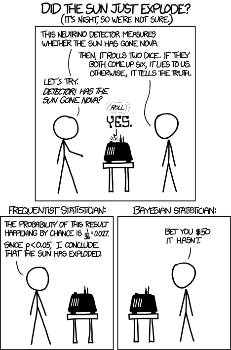
https://xkcd.com/1132/
Bayesian statistics derivation
Bayes’ theorem may be derived from the definition of conditional probability: \[P(A\mid B)={\frac {P(B\mid A)\,P(A)}{P(B)}},\;\text{if}\; P(B)\neq 0\] because \[P(B\cap A) = P(A\cap B)\] \[\Rightarrow P(A\cap B)=P(A\mid B)\,P(B)=P(B\mid A)\,P(A)\] \[\Rightarrow P(A\mid B)={\frac {P(B\mid A)\,P(A)}{P(B)}},\;\text{if}\; P(B)\neq 0\]
Classic example: Binomial experiment
- Given a sequence of coin tosses \(x_1, x_2, \ldots, x_M\), we want to estimate the (unknown) probability of heads: \[P(H) = \theta\]
- The instances are independent and identically distributed samples
Likelihood function
- How good is a particular parameter?
- Answer: Depends on how likely it is to generate the data \[L(\theta; D) = P(D\mid\theta) = \prod_m P(x_m \mid\theta)\]
- Example: Likelihood for the sequence: H, H, T, H, H \[L(\theta; D) = \theta \theta (1-\theta)\theta\theta = \theta^4 (1-\theta)\]

Maximum Likelihood Estimate (MLE)
- Choose parameters that maximize the likelihood function
- Commonly used estimator in statistics
- Intuitively appealing
- In the binomial experiment, MLE for probability of heads: \[\hat{\theta} = \frac{N_H}{N_H + N_T}\]
Is MLE the only option?
- Suppose that after 10 observations, MLE estimates the probability of a heads is 0.7.
- Would you bet on heads for the next toss?
- How certain are you that the true parameter value is 0.7?
- Were there enough samples for you to be certain?
Bayesian approach
- Formulate knowledge about situation probabilistically
- Define a model that expresses qualitative aspects of our knowledge (e.g., distributions, independence assumptions)
- Specify a prior probability distribution for unknown parameters that expresses our beliefs
- Compute the posterior probability distribution for the parameters, given observed data
- The posterior distribution can be used for:
- Reaching conclusions while accounting for uncertainty
- Make predictions that account for our uncertainty
Posterior distribution
- The posterior distribution combines the prior distribution with the likelihood function using Bayes’ rule: \[P(\theta \mid D) = \frac{P(\theta) P(D\mid \theta)}{P(D)}\]
- The denominator is just a normalizing constant so you can simplify: \[\mathrm{Posterior} \propto \mathrm{Prior} \times \mathrm{Likelihood}\]
- Predictions can be made by integrating over the posterior: \[P(\mathrm{new data} \mid D) = \int_{\theta} P(\mathrm{new data} \mid \theta) P(\theta \mid D) \delta \theta\]
Revisiting the Binomial experiment
- Prior distribution: uniform for \(\theta\) in [0, 1]
- Posterior distribution: \(P(\theta\mid x_1, \ldots ,x_M) \propto P(x_1, \ldots ,x_M\mid\theta)\times 1\)
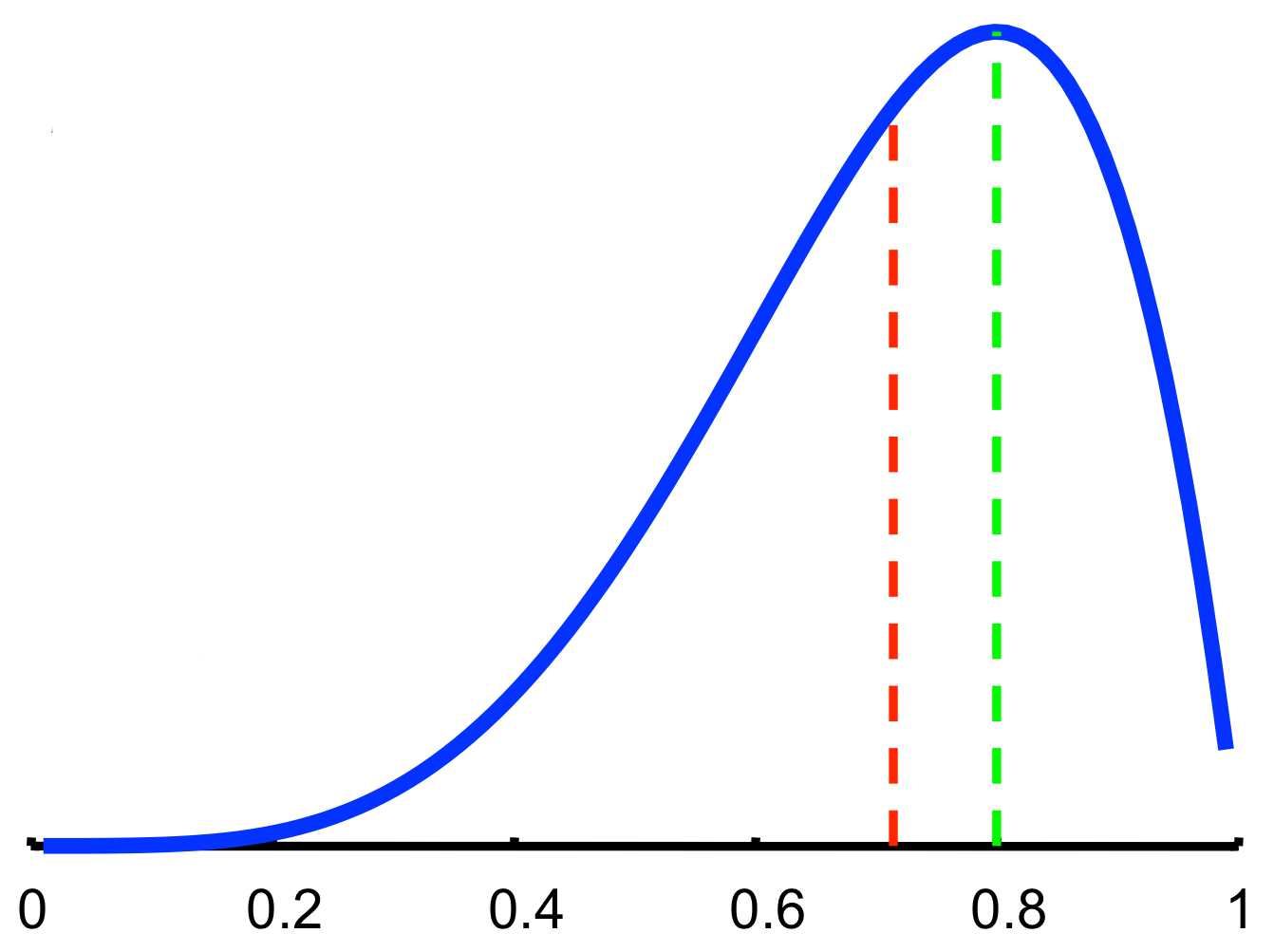
- Example: 5 coin tosses with 4 heads, 1 tail
- MLE estimate: \(P(\theta) = \tfrac{4}{5} = 0.8\)
- Bayesian prediction: \(P(x_{M+1}=H\mid D) = \int\theta P(\theta\mid D)\; d\theta = \tfrac{5}{7}\)
Bayesian inference and MLE
- The MLE and Bayesian prediction always differ in practice.
- However…
- If prior is well-behaved (i.e., does not assign 0 density to any “feasible” parameter value)
- Then both the MLE and Bayesian predictions converge to the same value as the training data becomes infinitely large
Features of the Bayesian approach
- Probability is used to describe “physical” randomness and uncertainty regarding the true values of the parameters.
- The prior and posterior probabilities represent degrees of belief, before and after seeing the data, respectively.
- The model and prior are chosen based on the knowledge of the problem and not, in theory, by the amount of data collected or the question we are interested in answering.
How to choose a prior
- Objective priors: Noninformative priors that attempt to capture ignorance.
- Subjective priors: Priors that capture our beliefs as completely as possible. They are subjective but not arbitrary.
- Hierarchical priors: Multiple levels of priors.
- Empirical priors: Learn some of the parameters of the prior from the data (“Empirical Bayes”)
- Robust, able to overcome limitations of mis-specification of prior
- Double counting of evidence / overfitting
Conjugate prior
- If the posterior distribution are in the same family as prior probability distribution, the prior and posterior are called conjugate distributions
- All members of the exponential family of distributions have conjugate priors
| Likelihood | Conjugate prior distribution | Prior hyperparameter | Posterior hyperparameters |
|---|---|---|---|
| Bernoulli | Beta | \(\alpha, \beta\) | \(\alpha + \sum x_i, \beta + n - \sum x_i\) |
| Multinomial | Dirichlet | \(\alpha\) | \(\alpha + \sum x_i\) |
| Poisson | Gamma | \(\alpha, \beta\) | \(\alpha + \sum x_i, \beta + n\) |
Computing the posterior distribution
- Analytical integration
- Works when “conjugate” prior distributions can be used, which combine nicely with the likelihood—usually not the case.
- Gaussian approximation
- Works well when there is sufficient data compared to model complexity—posterior distribution is close to Gaussian (Central Limit Theorem) and can be handled by finding its mode.
- Markov chain Monte Carlo
- Simulate a Markov chain that eventually converges to the posterior distribution—currently the dominant approach.
- Variational approximation
- Cleverer way to approximate the posterior and maybe faster than MCMC but not as general and exact.
Limitations and criticisms of Bayesian methods
- It is hard to come up with a prior (subjective) and the assumptions may be wrong
- Closed world assumption: need to consider all possible hypotheses for the data before observing the data
- Computationally demanding (compared to frequentist approach)
- Use of approximations weakens coherence argument
Example: Diagnostic testing
Facts:
- Rapid home tests will pick up an HIV infection 97.7% of the time 28 days after exposure (sensitivity).
- These same tests have a specificity of 95%.
- 0.34% of the US population is estimated to be infected.
Questions:
- A US resident receives a positive test. What is the chance they have HIV?
- How would this change if 5% of the population were infected?
Reading & Resources
- 📖: Bayesian Data Analysis
- 📖: Probabilistic Programming & Bayesian Methods for Hackers
- 📺: Bayes theorem, the geometry of changing beliefs
- 📺: The medical test paradox, and redesigning Bayes’ rule
- 👂: Linear Digressions: Beware of simple metrics
- Software packages for Bayesian analysis:
Review Questions
- What is a prior? How does one go about making one?
- Can a prior be based on data? If so, how is this data related to the experiment being modeled (the observed)?
- What are three differences between a Bayesian and maximum likelihood (frequentist) approach?
- When will a Bayesian and maximum likelihood approach agree?
- You are asked to provide up-to-date estimates of the 6-month failure rate for a stent going to market. A previous device had 3 devices out of 100 fails within 6 months, and you strongly suspect this device is similar. Provide the Bayesian estimate of the failure rate (i.e. \(P(FR \vert N,m))\) given N devices have made it to 6 months, and m have failed. (Hint: Devices either pass or fail here. This follows a Binomial distribution.)
- What would be a reasonable estimate if you had no previous device’s data?
- What do you expect to happen to a posterior distribution as you add more and more data?
- What does the integral of \(p(a \vert b) p(b \vert c) \delta b\) give you? Why is this useful?