Dimensionality Reduction: PCA and NMF
Dealing with many variables
- So far we’ve largely concentrated on cases in which we have relatively large numbers of measurements for a few variables
- This is frequently refered to as \(n > p\)
- Two other extremes are imporant
- Many observations and many variables
- Many variables but few observations (\(p > n\))
Dealing with many variables
Usually when we’re dealing with many variables, we don’t have a great understanding of how they relate to each other
- E.g. if gene X is high, we can’t be sure that will mean gene Y will be too
- If we had these relationships, we could reduce the data
- E.g. if we had variables to tell us it’s 3 pm in Los Angeles, we don’t need one to say it’s daytime
Dimensionality Reduction
Generate a low-dimensional encoding of a high-dimensional space
Purposes:
- Data compression / visualization
- Robustness to noise and uncertainty
- Potentially easier to interpret
Bonus: Many of the other methods from the class can be applied after dimensionality reduction with little or no adjustment!
Matrix Factorization
Many dimensionality reduction methods involve matrix factorization
Basic Idea: Find two (or more) matrices whose product best approximate the original matrix
Low rank approximation to original \(N\times M\) matrix:
\[ \mathbf{X} \approx \mathbf{W} \mathbf{H}^{T} \]
where \(\mathbf{W}\) is \(N\times R\), \(\mathbf{H}^{T}\) is \(M\times R\), and \(R \ll N\).
Matrix Factorization

Generalization of many methods (e.g., SVD, QR, CUR, Truncated SVD, etc.)
Aside - What should R be?
\[ \mathbf{X} \approx \mathbf{W} \mathbf{H}^{T} \]
where \(\mathbf{W}\) is \(M\times R\), \(\mathbf{H}^{T}\) is \(M\times R\), and \(R \ll N\).
Matrix factorization is also compression

https://www.aaronschlegel.com/image-compression-principal-component-analysis/
Matrix factorization is also compression

https://www.aaronschlegel.com/image-compression-principal-component-analysis/
Matrix factorization is also compression

https://www.aaronschlegel.com/image-compression-principal-component-analysis/
Examples
Process control
- Large bioreactor runs may be recorded in a database, along with a variety of measurements from those runs
- We may be interested in how those different runs varied, and how each factor relates to one another
- Plotting a compressed version of that data can indicate when an anomolous change is present
Mutational processes
- Anytime multiple contributory factors give rise to a phenomena, matrix factorization can separate them out
- Will talk about this in greater detail
Cell heterogeneity
- Enormous interest in understanding how cells are similar or different
- Answer to this can be in millions of different ways
- But cells often follow programs
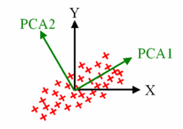
Principal Components Analysis
Principal Components Analysis
- Each principal component (PC) is linear combination of uncorrelated attributes / features’
- Ordered in terms of variance
- \(k\)th PC is orthogonal to all previous PCs
- Reduce dimensionality while maintaining maximal variance
Methods to calculate PCA
- All methods are essentially deterministic
- Iterative computation
- More robust with high numbers of variables
- Slower to calculate
- NIPALS (Non-linear iterative partial least squares)
- Able to efficiently calculate a few PCs at once
- Breaks down for high numbers of variables (large p)
Practical notes
- Implemented within
sklearn.decomposition.PCAPCA.fit_transform(X)fits the model toX, then provides the data in principal component spacePCA.components_provides the “loadings matrix”, or directions of maximum variancePCA.explained_variance_provides the amount of variance explained by each component
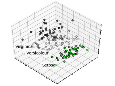
Code example
import matplotlib.pyplot as plt
from sklearn import datasets
from sklearn.decomposition import PCA

iris = datasets.load_iris()

X = iris.data
y = iris.target
target_names = iris.target_names

pca = PCA(n_components=2)
X_r = pca.fit(X).transform(X)

# Print PC1 loadings
print(pca.components_[:, 0])

# Print PC1 scores
print(X_r[:, 0])

# Percentage of variance explained for each component
print(pca.explained_variance_ratio_)
# [ 0.92461621  0.05301557]
Separating flower species
Non-negative matrix factorization
What if we have data wherein effects always accumulate?
Application: Mutational processes in cancer
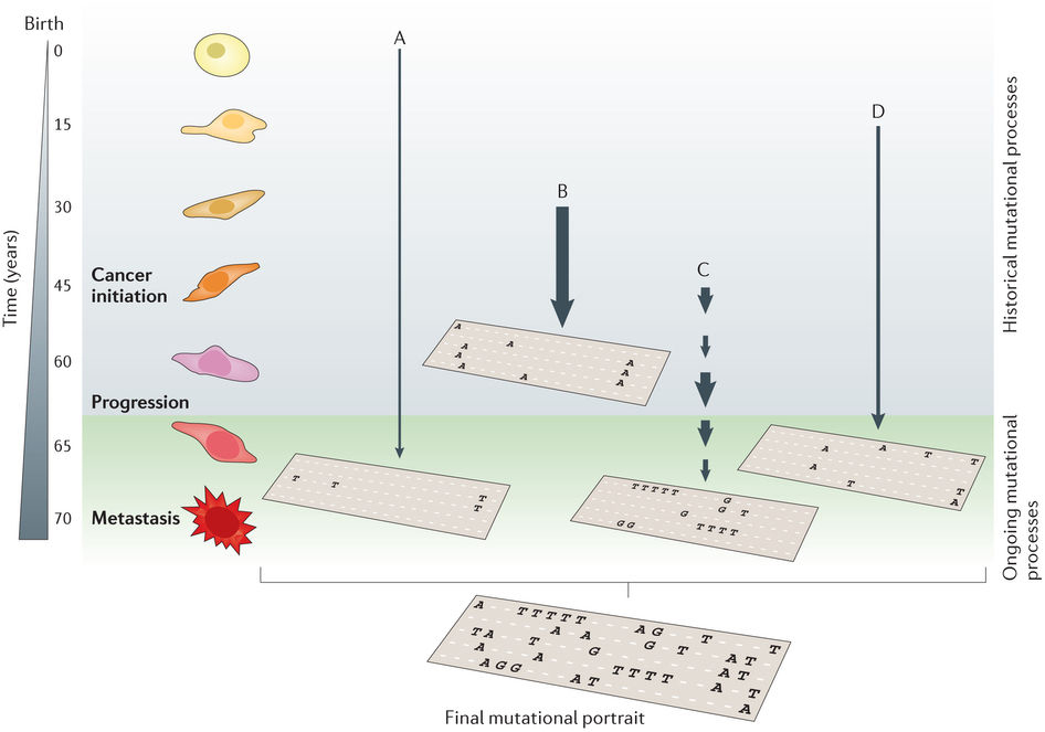
Helleday et al, Nat Rev Gen, 2014
Helleday et al, Nat Rev Gen, 2014
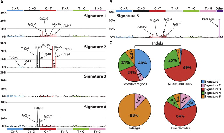
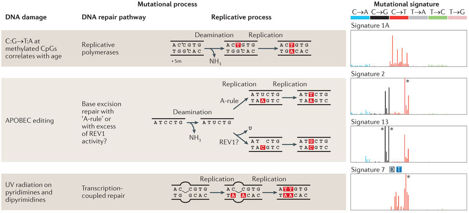
Alexandrov et al, Cell Rep, 2013
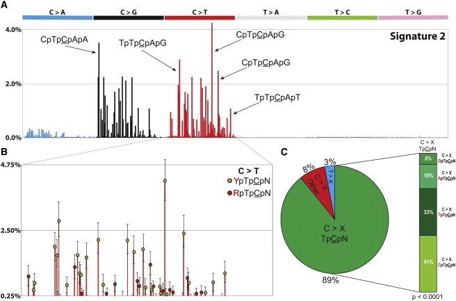
Alexandrov et al, Cell Rep, 2013
Important considerations
- Like PCA, except the coefficients must be non-negative
- Forcing positive coefficients implies an additive combination of parts to reconstruct whole
- Leads to sparse factors
- The answer you get will always depend on the error metric, starting point, and search method
Multiplicative update algorithm
- The update rule is multiplicative instead of additive
- In the initial values for W and H are non-negative, then W and H can never become negative
- This guarantees a non-negative factorization
- Will converge to a local maxima
- Therefore starting point matters
Multiplicative update algorithm: Updating W
\[[W]_{ij} \leftarrow [W]_{ij} \frac{[\color{darkred} X \color{darkblue}{H^T} \color{black}]_{ij}}{[\color{darkred}{WH} \color{darkblue}{H^T} \color{black}]_{ij}}\]
Color indicates the reconstruction of the data and the projection matrix.
Multiplicative update algorithm: Updating H
\[[H]_{ij} \leftarrow [H]_{ij} \frac{[\color{darkblue}{W^T} \color{darkred}X \color{black}]_{ij}}{[\color{darkblue}{W^T} \color{darkred}{WH} \color{black}]_{ij}}\]
Color indicates the reconstruction of the data and the projection matrix.
Coordinate descent solving
- Another approach is to find the gradient across all the variables in the matrix
- Not going to go through implementation
- Will also converge to a local maxima
Practical notes
- Implemented within
sklearn.decomposition.NMF.n_components: number of componentsinit: how to initialize the searchsolver: ‘cd’ for coordinate descent, or ‘mu’ for multiplicative updatel1_ratio,alpha_H,alpha_W: Can regularize fit
- Provides:
NMF.components_: components x features matrix- Returns transformed data through
NMF.fit_transform()
Summary
PCA
- Preserves the covariation within a dataset
- Therefore mostly preserves axes of maximal variation
- Number of components will vary in practice
NMF
- Explains the dataset through two non-negative matrices
- Much more stable patterns when assumptions are appropriate
- Will explain less variance for a given number of components
- Excellent for separating out additive factors
Closing
As always, selection of the appropriate method depends upon the question being asked.
Reading & Resources
Review Questions
- What do dimensionality reduction methods reduce? What is the tradeoff?
- What are three benefits of dimensionality reduction?
- Does matrix factorization have one answer? If not, what are two choices you could make?
- What does principal components analysis aim to preserve?
- What are the minimum and maximum number of principal components one can have for a dataset of 300 observations and 10 variables?
- How can you determine the “right” number of PCs to use?
- What is a loading matrix? What would be the dimensions of this matrix for the dataset in Q5 when using three PCs?
- What is a scores matrix? What would be the dimensions of this matrix for the dataset in Q5 when using three PCs?
- By definition, what is the direction of PC1?
- See question 5 on midterm W20. How does movement of the siControl EGF point represent changes in the original data?