Support Vector Machines
Aaron Meyer (adapted from slides by Martin Law)
History Of SVM
- SVM is related to statistical learning theory
- First introduced in 1992
- Became popular because of its success in handwritten digit recognition
- 1.1% test error rate for SVM. Same error as a perceptron model.
- Also used in very first self-driving cars
- Later bested by deep learning methods
- Note: the meaning of “kernel” is different from other methods
Application

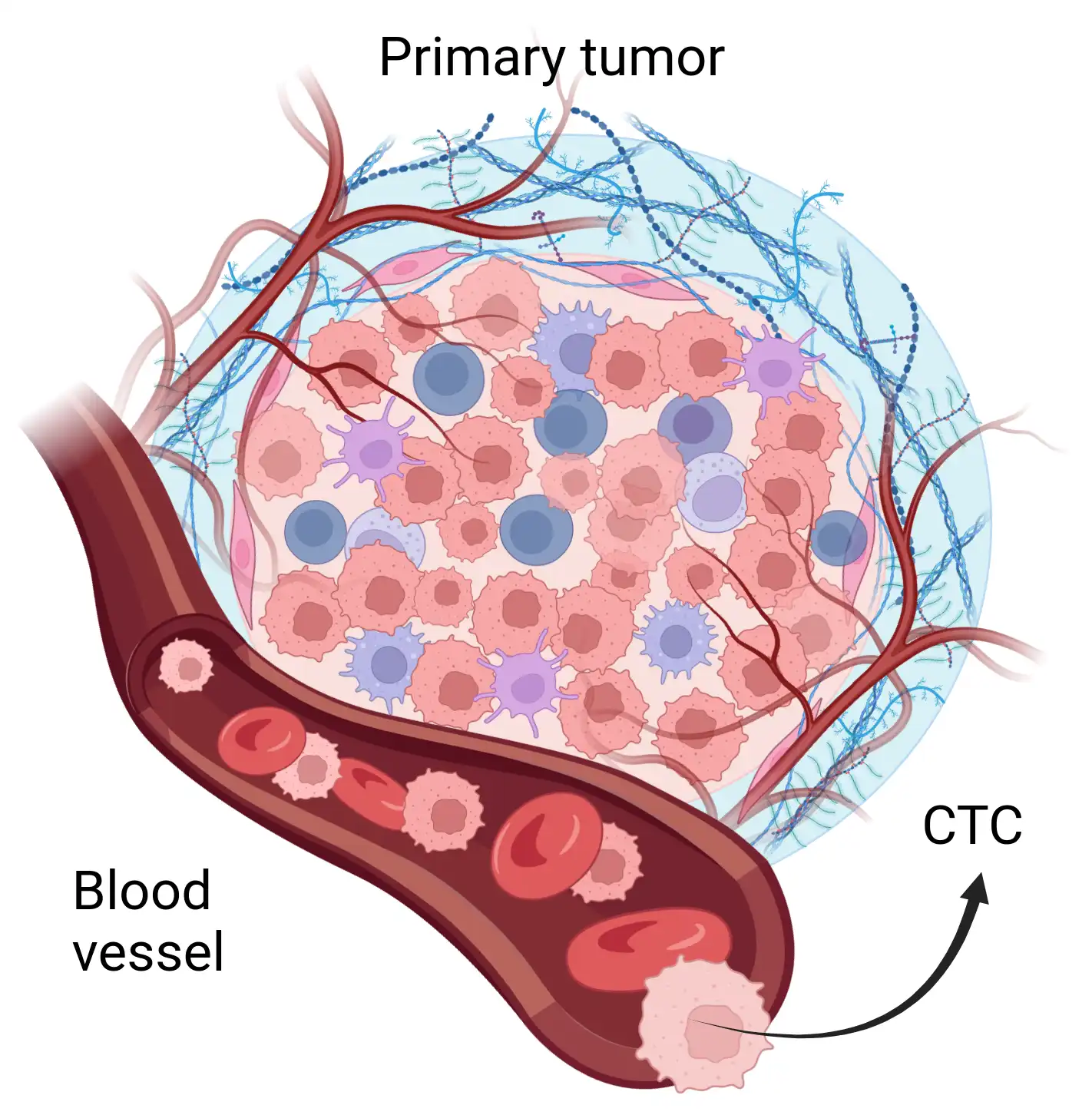
CTCs enable assessment of patient state and drug response
- Found in the blood of metastatic cancer patients
- Approximately 1 CTC per billion blood cells
- CTs have great clinical value
- Liquid biopsy
- Genetic information
- Prognostic
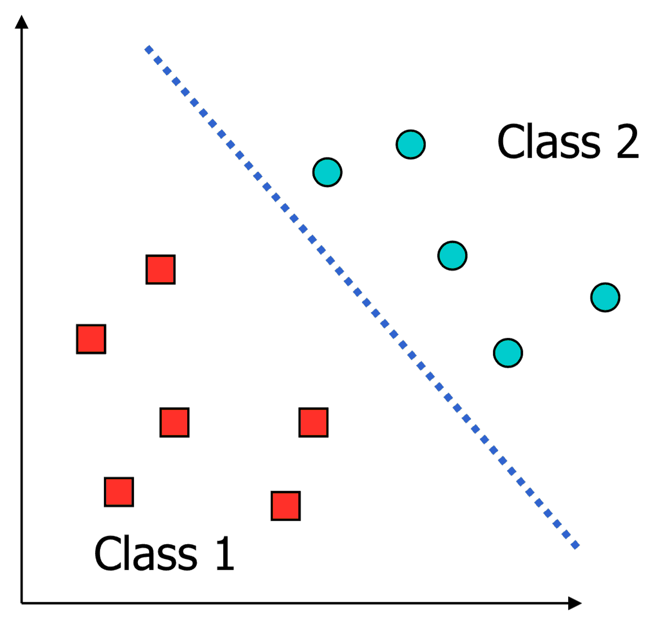
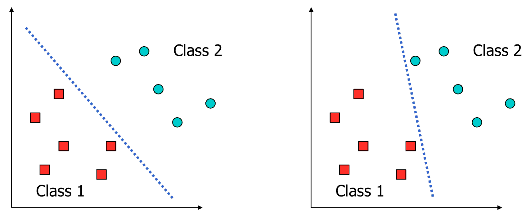
What is a good decision boundary?
Consider a two-class, linearly separable classification problem
Examples Of Bad Decision Boundaries
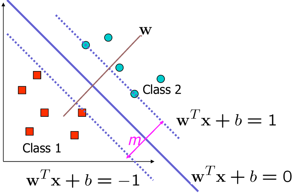
Large-Margin Decision Boundary
- The decision boundary should be as far away from the data of both classes as possible
- We should maximize the margin, \(m = 2 / \lVert \mathbf{w} \rVert\)
- Distance between the origin and the line \(\mathbf{w}^T\mathbf{x}=k\) is \(k / \lVert \mathbf{w} \rVert\)
Finding The Decision Boundary
- Let \(\{x_1, \ldots, x_n\}\) be our data set and let \(y_i \in \{1, -1\}\) be the class label of \(x_i\)
- The decision boundary should classify all points correctly
- \(y_i \left(\mathbf{w}^T \mathbf{x}_i + b\right) \ge 1, \quad \forall i\)
- The decision boundary can be found by solving the following constrained optimization problem:
- Minimize \(\frac{1}{2}\lVert \mathbf{w} \rVert^2\)
- subject to \(y_i \left(\mathbf{w}^T \mathbf{x}_i + b\right) \ge 1\)
- This is a constrained optimization problem
- Quick methods to find the global optimum by quadratic programming
The Quadratic Programming Problem
Many approaches have been proposed
- Most are “interior-point” methods
- Start with an initial solution that can violate the constraints
- Improve this solution by optimizing the objective function and/or reducing the amount of constraint violation
- For SVM, sequential minimal optimization is most popular
- A QP with two variables is trivial to solve
- Each iteration of SMO picks a pair of (\(\alpha_i, \alpha_j\)) and solve the QP with these two variables; repeat until convergence
- In practice, we can just regard the QP solver as a “black-box” without bothering how it works
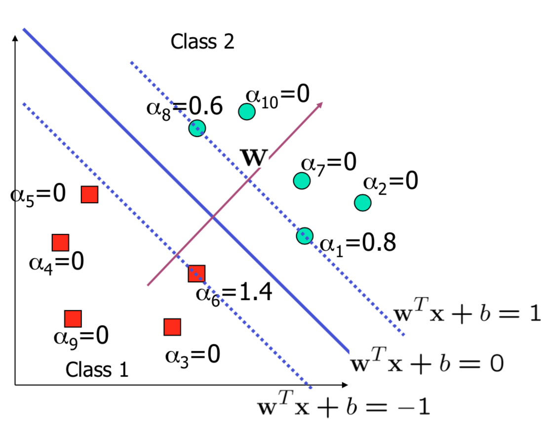
Characteristics of the solution
- \(x_i\) with non-zero \(\alpha_i\) are called support vectors (SV)
- The decision boundary is determined only by the SV
- Let \(t_j (j=1, \ldots, s)\) be the indices of the \(s\) support vectors
- We can write \(\mathbf{w} = \sum_{j=1}^{s} \alpha_{t_{j}}y_{t_{j}}\mathbf{x}_{t_{j}}\)
- Many \(\alpha_i\) are zero!
- \(w\) is a linear combination of a small number of data points
- This “sparse” representation can be viewed as data compression
- For testing with a new data \(z\)
- Compute \(\mathbf{w}^T \mathbf{z} + b = \sum_{j=1}^{s} \alpha_{t_{j}}y_{t_{j}}\left( \mathbf{x}_{t_{j}}^T \mathbf{z} \right) + b\)
- Classify \(z\) as class 1 if the sum is positive, and class 2 otherwise
- Note: \(w\) need not be formed explicitly
A geometrical interpretation
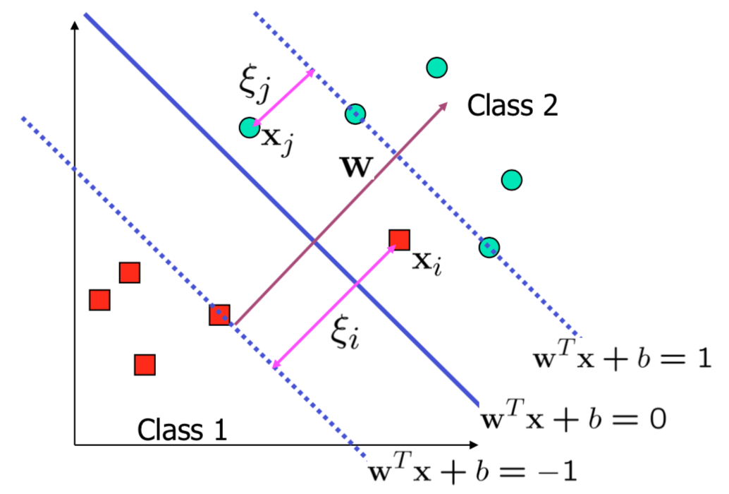
Non-linearly-separable problems
What can we do when we can’t draw a line that separates the two classes?
Non-linearly-separable problems
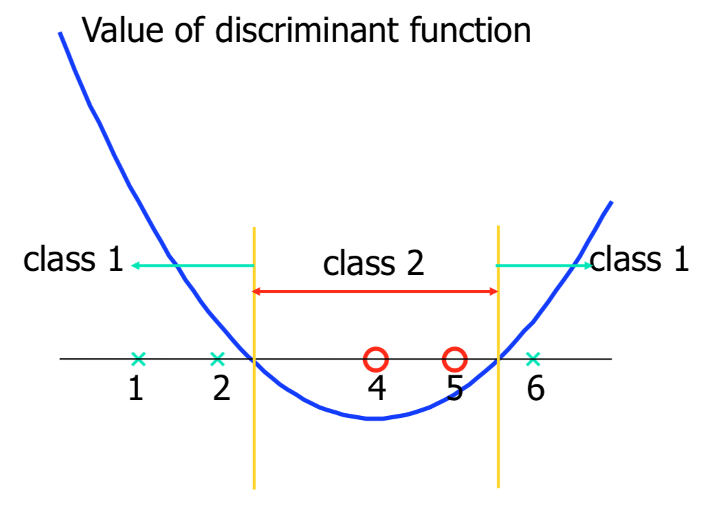
- We allow “error” \(\xi_i\) in classification; it is based on the output of the discriminant function \(\mathbf{w}^T\mathbf{x} + b\)
- \(\xi_i\) approximates the number of misclassified samples
Soft margin hyperplane
- If we minimize \(\sum_i \xi_i\), \(\xi_i\) can be computed by
- \((\mathbf{w}^T \mathbf{x}_i + b) \geq 1 - \xi_i \quad y_i = 1\)
- \((\mathbf{w}^T \mathbf{x}_i + b) \leq -1 + \xi_i \quad y_i = -1\)
- \(\xi_i \geq 0\)
- \(\xi_i\) are “slack variables” in optimization
- Note that \(\xi_i = 0\) if there is no error for \(\mathbf{x}_i\)
- \(\xi_i\) is an upper bound of the number of errors
- We want to minimize:
- \(\tfrac{1}{2} \lVert \mathbf{w} \rVert^2 + C \sum_{i=1}^{n} \xi_i\)
- \(C\): tradeoff parameter between error and margin
Soft margin hyperplane
- The optimization problem becomes:
- Minimize \(\tfrac{1}{2} \lVert \mathbf{w} \rVert^2 + C \sum_{i=1}^{n} \xi_i\)
- subject to \(y_i (\mathbf{w}^T \mathbf{x}_i + b) \geq 1 - \xi_i, \quad \xi_i \geq 0\)
The optimization problem
- The dual of this new constrained optimization problem is:
- max. \(W(\alpha) = \sum_{i=1}^n \alpha_i - \frac{1}{2} \sum_{i=1,j=1}^n \alpha_i \alpha_j y_i y_j \mathbf{x}_i^T \mathbf{x}_j\)
- subject to \(C \geq \alpha_i \geq 0, \sum_{i=1}^n \alpha_i y_i = 0\)
- w is recovered as \(\mathbf{w} = \sum_{j=1}^s \alpha_{t_j} y_{t_j} \mathbf{x}_{t_j}\)
- This is very similar to the optimization problem in the linear separable case, except that there is an upper bound \(C\) on \(\alpha_i\) now
- Once again, a QP solver can be used to find \(\alpha_i\)
Extension to a non-linear decision boundary
Non-linear decision boundaries
- So far, we have only considered large-margin classifier with a linear decision boundary
- How to generalize it to become nonlinear?
- Key idea: transform \(\mathbf{x}_i\) to a higher dimensional space to “make life easier”
- Input space: the space the point \(\mathbf{x}_i\) are located
- Feature space: the space of \(\phi(\mathbf{x}_i)\) after transformation
- Why transform?
- Linear operation in the feature space is equivalent to non-linear operation in input space
- Classification can become easier with a proper transformation.
Transforming The Data
- Note that feature space is usually of higher dimensions in practice
- Computation in the feature space can be costly because it is high dimensional
- The feature space is typically infinite-dimensional!
- The kernel trick comes to rescue
The kernel trick
- Recall the SVM optimization problem
- The data points only appear as the inner product
- max. \(W(\alpha) = \sum_{i=1}^n \alpha_i - \frac{1}{2} \sum_{i=1,j=1}^n \alpha_i \alpha_j y_i y_j \mathbf{x}_i^T \mathbf{x}_j\)
- subject to \(C \geq \alpha_i \geq 0, \sum_{i=1}^n \alpha_i y_i = 0\)
- As long as we can calculate the inner product in the feature space, we do not need the mapping explicitly
- Many common geometric operations (angles, distances) can be expressed by inner products
- Define the kernel function \(K\) by: \[K(x_i, x_j) = \phi \left(x_i\right)^T \phi \left(x_j\right)\]
Kernel Functions
- In practical use of SVM, the user specifies the kernel function; the transformation φ(.) is not explicitly stated
- Given a kernel function \(K(x_i, x_j)\), the transformation \(\phi(.)\) is given by its eigenfunctions (a concept in functional analysis)
- Eigenfunctions can be difficult to construct explicitly
- This is why people only specify the kernel function without worrying about the exact transformation
- Another view: kernel function, being an inner product, is really a similarity measure between the objects
Examples of Kernel Functions
- Polynomial kernel with degree \(d\)
- \(K(\mathbf{x},\mathbf{y}) = \left( \mathbf{x}^T \mathbf{y} + 1 \right)^d\)
- Radial basis function kernel with width \(\sigma\)
- \(K(\mathbf{x},\mathbf{y}) = \exp (-\lVert \mathbf{x} - \mathbf{y} \rVert^2 / (2\sigma^2))\)
- Closely related to radial basis function neural networks
- The feature space is infinite-dimensional
- Sigmoid with parameter \(\kappa\) and \(\theta\)
- \(K(\mathbf{x},\mathbf{y}) = \tanh (\kappa \mathbf{x}^T \mathbf{y} + \theta)\)
Modification Due to Kernel Function
- Change all inner products to kernel functions
- For training:
- Original: max. \(W(\alpha) = \sum_{i=1}^n \alpha_i - \frac{1}{2} \sum_{i=1,j=1}^n \alpha_i \alpha_j y_i y_j \mathbf{x}_i^T \mathbf{x}_j\)
- With kernel function: max. \(W(\alpha) = \sum_{i=1}^n \alpha_i - \frac{1}{2} \sum_{i=1,j=1}^n \alpha_i \alpha_j y_i y_j K\left( \mathbf{x}_i^T \mathbf{x}_j \right)\)
- Both: subject to \(C \geq \alpha_i \geq 0, \sum_{i=1}^n \alpha_i y_i = 0\)
Modification Due to Kernel Function
- For testing, the new data \(z\) is classified as:
- class 1 if \(f \geq 0\)
- class 2 if \(f < 0\)
- Original:
- \(\mathbf{w} = \sum_{j=1}^{s} \alpha_{t_{j}}y_{t_{j}}\mathbf{x}_{t_{j}}\)
- \(f = \mathbf{w}^T \mathbf{z} + b = \sum_{j=1}^{s} \alpha_{t_{j}}y_{t_{j}}\left( \mathbf{x}_{t_{j}}^T \mathbf{z} \right) + b\)
- With kernel function:
- \(\mathbf{w} = \sum_{j=1}^{s} \alpha_{t_{j}}y_{t_{j}} \phi\left(\mathbf{x}_{t_{j}}\right)\)
- \(f = \langle \mathbf{w}, \phi\left(\mathbf{z}\right) \rangle + b = \sum_{j=1}^{s} \alpha_{t_{j}}y_{t_{j}}K\left( \mathbf{x}_{t_{j}}^T, \mathbf{z} \right) + b\)
More on Kernel Functions
- Since the training of SVM only requires the value of \(K(\mathbf{x}_i, \mathbf{x}_j)\), there is no restriction of the form of \(\mathbf{x}_i\) and \(\mathbf{x}_j\)
- \(\mathbf{x}_i\) can be a sequence or a tree, instead of a feature vector
- \(K(\mathbf{x}_i, \mathbf{x}_j)\) is just a similarity measure comparing \(\mathbf{x}_i\) and \(\mathbf{x}_j\)
- For a test object \(z\), the discrimination function essentially is a weighted sum of the similarity between \(z\) and a pre-selected set of objects (the support vectors):
- \(f(\mathbf{z}) = \sum_{\mathbf{x}_i \in S}\alpha_i y_i K(\mathbf{z}, \mathbf{x}_i) + b\)
- \(S\): the set of support vectors
Example of Non-Linear Transformation
Justification of SVM
- Large margin classifier
- Ridge regression: the term \(\tfrac{1}{2}\lVert w \rVert^2\) “shrinks” the parameters towards zero to avoid overfitting
- The term the term \(\tfrac{1}{2}\lVert w \rVert^2\) can also be viewed as imposing a weight-decay prior on the weight vector
Choosing the Kernel Function
- Probably the most tricky part of using SVM
- The kernel function is important because it creates the kernel matrix, which summarizes all the data
- In practice, a low degree polynomial kernel or RBF kernel with a reasonable width is a good initial try
Other Aspects of SVM
- How to use SVM for multi-class classification?
- One can change the QP formulation to become multi-class
- More often, multiple binary classifiers are combined
- One can train multiple one-versus-all classifiers, or combine multiple pairwise classifiers “intelligently”
- How to interpret the SVM discriminant function value as probability?
- By performing logistic regression on the SVM output of a set of data (validation set) that is not used for training
Summary
Classification steps
- Prepare the pattern matrix
- Select the kernel function to use
- Select the parameter of the kernel function and the value of C
- You can use the values suggested by the SVM software, or you can set apart a validation set to determine the values of the parameter
- Execute the training algorithm and obtain the \(\alpha_i\)
- Unseen data can be classified using the \(\alpha_i\) and the support vectors
Strengths and weaknesses of SVM
- Strengths
- Training is relatively easy (no local optima, unlike in neural networks)
- Scales well to high-dimensional data
- Complexity versus error can be controlled
- Non-traditional data like strings and trees can be used as input to SVM, instead of feature vectors
- Weaknesses
- Need to choose a “good” kernel function.
- Not generative
- Difficult to interpret
- Need fully labelled data
Other types of kernel methods
- Key lesson: a linear algorithm in the feature space is equivalent to a non-linear algorithm in the input space
- Standard linear algorithms can be generalized to its non-linear version by going to the feature space
- Kernel principal component analysis, kernel independent component analysis, kernel canonical correlation analysis, kernel k-means, 1-class SVM are some examples
Multi-class classification
- SVM is basically a two-class classifier
- One can change the QP formulation to allow multi-class classification
- More commonly, one splits the classes into binary decisions
Implementation
sklearn has implementations for a variety of SVM methods:
sklearn.svm.SVC- Performs single or multi-class classification
- Multi-class is through one-vs-one scheme
- Multiple kernels available
linear: \(\langle x, x'\rangle\)polynomial: \((\gamma \langle x, x'\rangle + r)^d\)rbf: \(\exp(-\gamma \|x-x'\|^2)\)sigmoid: \(\tanh(\gamma \langle x,x'\rangle + r)\)
- Performs single or multi-class classification
- Alternative implementations
sklearn.svm.NuSVC- Additionally provides parameter to control number of support parameters
sklearn.svm.LinearSVC- Only support for linear kernel, with better scaling/options
- For example can provide l1 or l2 regularization
- Scales better for many samples
Reading & Resources
Review Questions
- What is the core observation underlying SVMs?
- Does the answer for an SVM rely on the exact position of all points? If not, which points most influence the model?
- Where can you find the support vectors in a dataset?
- What is a kernel? What are three common kinds?
- Can you use SVMs for data that can’t be perfectly separated? What do you do if so? What additional tradeoff does this create?
- What is a hyperparameter? How do you find the value of these?
- How is Y represented within an SVM model?
- You use an SVM model with an RBF kernel and a high value for gamma. What does the value of gamma indicate?
- When the C parameter is set to be infinite, which of the following is true?
- Your colleague is using an SVM with poly kernel and notices that the fitting error improves with ever higher degree polynomials. What is happening here? What would you suggest they do?
- Can an SVM model be used with more than two classes? If so, how?