where \(\mathbf{W}\) is \(N\times R\), \(\mathbf{H}\) is \(M\times R\), and \(R \ll \min(N, M)\).
Visualizing matrix factorization
Visualization of matrix factorization, showing a data matrix X approximated by the product of W and H transpose, with sample and feature axes and common names for the factor matrices in PCA and NMF.
Generalization of many methods (e.g., SVD, QR, CUR, Truncated SVD, etc.)
Often scale each feature to unit variance when variables are in different units
Otherwise a high-variance measurement can dominate PC1
Any new samples must be transformed using the same centering and scaling learned from the training data
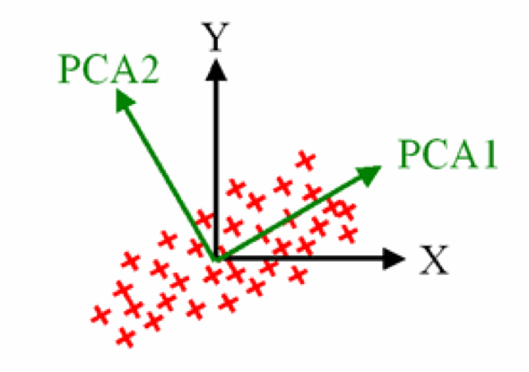
PCA example: words
Consider an example dataset of two variables about words
The number of lines of its dictionary definition
The length of a word
Example from Abdi & Williams, 2010
We obtain \(\mathbf{X}\) after applying appropriate centering and normalization
PCA identifies two orthogonal axes of variation
The first component (PC1) explains the most variation
The second component (PC2) is orthogonal to PC1
One can project the observed data points onto the principal components
Scores for each data point
We can read the projected scores for each data point
Projecting new data with PCA
Once you have characterized the PCA components, you may use the loadings to project new data points.
PCA words example: projecting a new word, ‘sur’.
Score for the new word, ‘sur’.
PCA gives a low-rank approximation
PCA approximates the original data using only a few principal directions
Keeping the first \(R\) PCs gives the best rank-\(R\) linear approximation in least squares terms
Geometrically: project the data onto a lower-dimensional subspace, then reconstruct back into the original space
Visualization of PCA as a low-rank approximation: data points are approximated by projection onto the leading principal component directions.
Interpreting PCA outputs
Scores tell you where each observation lies in PC space
Loadings tell you which original features define each PC
Large-magnitude loadings indicate features that contribute strongly to that component
The sign of a PC is arbitrary
Flipping all scores and loadings for a component gives the same model
How many PCs should we keep?
Look at the explained variance ratio
Use a scree plot to look for an elbow
Keep enough PCs for the downstream goal
Visualization may need only 2-3 PCs
Denoising or compression may need more
Validate the choice with reconstruction error or downstream performance when possible
Algorithms: computing PCA
Classical PCA is often computed with an SVD or eigendecomposition
These are deterministic for a fixed input matrix
Iterative methods are also used in practice
Helpful for very large matrices or when only a few PCs are needed
NIPALS (nonlinear iterative partial least squares)
Able to efficiently calculate a few PCs without a full decomposition
Useful when the full SVD would be expensive
PCA in practice
Implemented within sklearn.decomposition.PCA
PCA.fit_transform(X) fits the model to X, then provides the data in principal component space
PCA.components_ provides the “loadings matrix”, or directions of maximum variance
PCA.explained_variance_ provides the amount of variance explained by each component
PCA.explained_variance_ratio_ gives the fraction of total variance explained by each PC
PCA code example
import matplotlib.pyplot as pltfrom sklearn import datasetsfrom sklearn.decomposition import PCAiris = datasets.load_iris()X = iris.datay = iris.targettarget_names = iris.target_namespca = PCA(n_components=2)X_r = pca.fit_transform(X)# Print PC1 loadingsprint(pca.components_[0, :])# Print PC1 scoresprint(X_r[:, 0])# Percentage of variance explained for each componentprint(pca.explained_variance_ratio_)# [ 0.92461621 0.05301557]
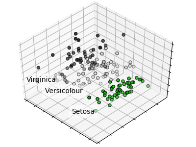
PCA example: separating flower species
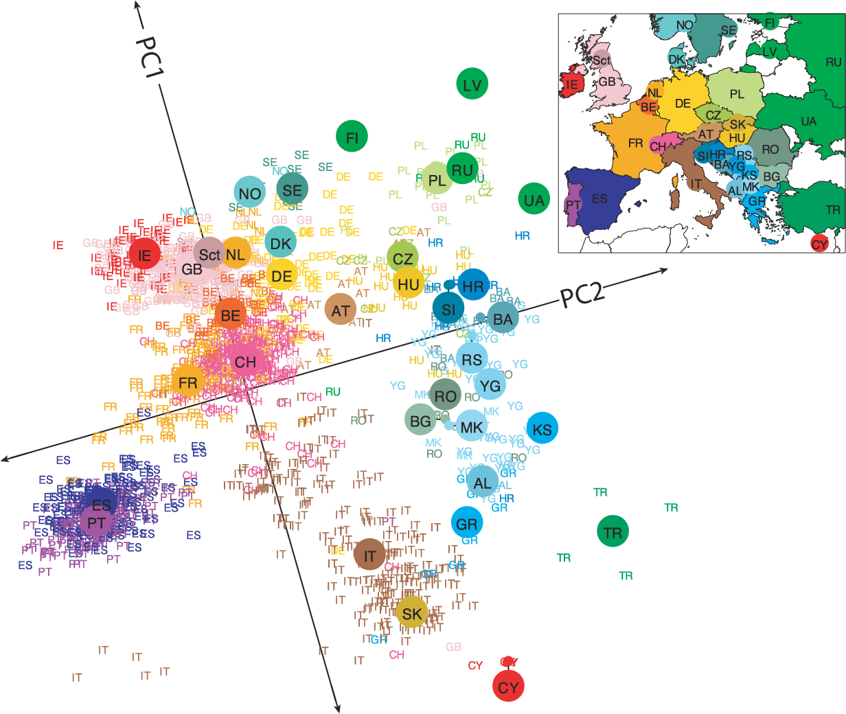
PCA example: genes mirror geography within Europe
A statistical summary of genetic data from 1,387 Europeans based on principal component axis one (PC1) and axis two (PC2). Novembre et al. Nature. 2008.
Non-Negative Matrix Factorization (NMF)
What if we have data wherein effects always accumulate?
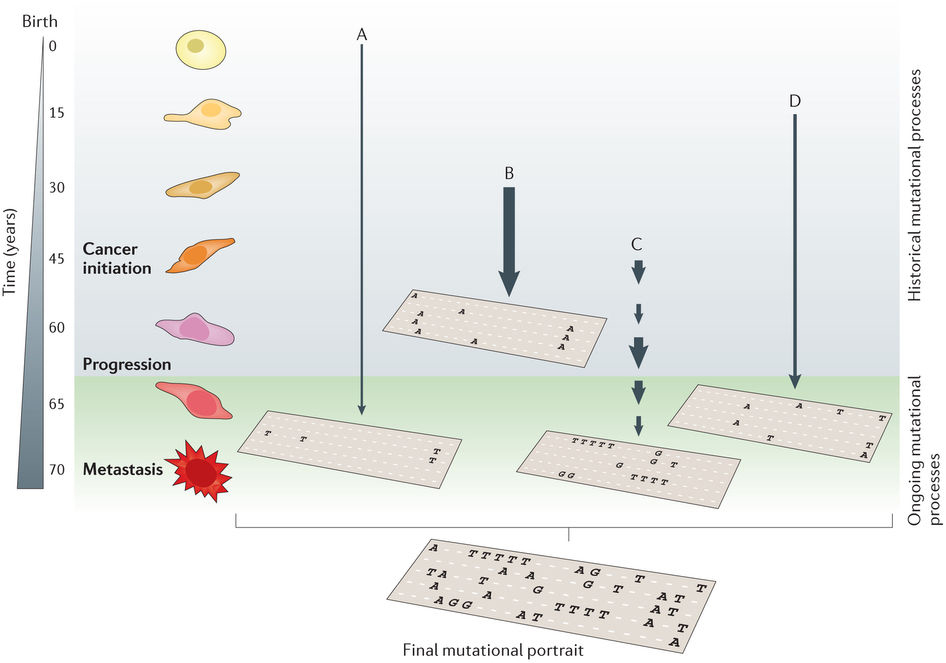
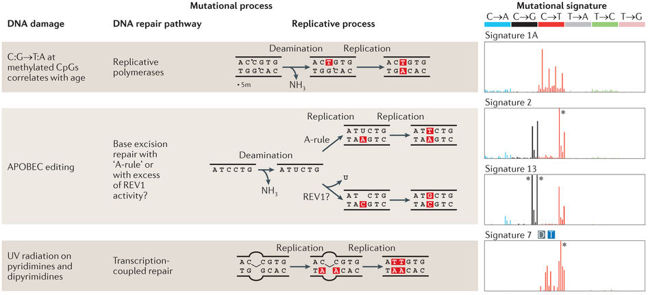
NMF application: mutational processes in cancer
Helleday et al, Nat Rev Gen, 2014
Helleday et al, Nat Rev Gen, 2014
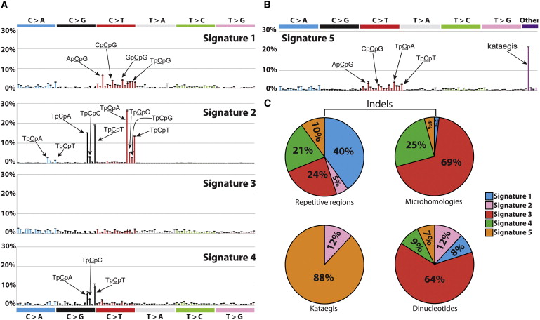
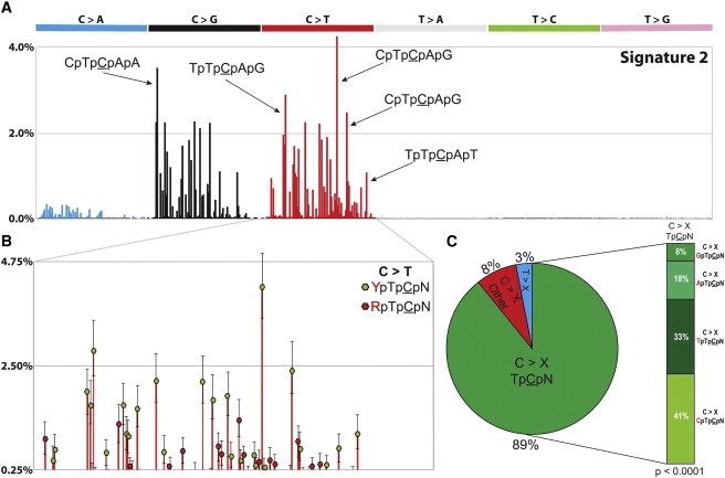
Alexandrov et al, Cell Rep, 2013
Alexandrov et al, Cell Rep, 2013
Important considerations
Like PCA, except the coefficients must be non-negative
Forcing positive coefficients implies an additive combination of parts to reconstruct the whole
Leads to sparse factors
The answer you get will always depend on the error metric, starting point, and search method
NMF objective
Find non-negative matrices \(\mathbf{W}\) and \(\mathbf{H}\) such that