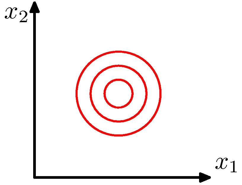
Circular distribution
\[P(X=\mathbf{x}_{j})=\frac{1}{(2\pi)^{m/2}\|\Sigma\|^{1/2}}\exp\left[-\frac{1}{2}(\mathbf{x}_{j}-\boldsymbol{\mu})^{T}\Sigma^{-1}(\mathbf{x}_{j}-\boldsymbol{\mu})\right]\]
\(\Sigma\) is the identity matrix
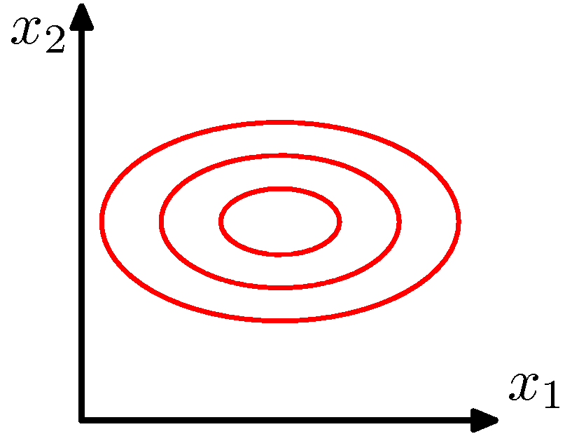
Ovals!
\[P(X=\mathbf{x}_j) = \frac{1}{(2\pi)^{m/2} \|\Sigma\|^{1/2}} \exp\left[-\frac{1}{2}(\mathbf{x}_j - \boldsymbol{\mu})^T \Sigma^{-1} (\mathbf{x}_j - \boldsymbol{\mu})\right]\]
\(\Sigma\) is a diagonal matrix
\(X_i\) are independent and uncorrelated
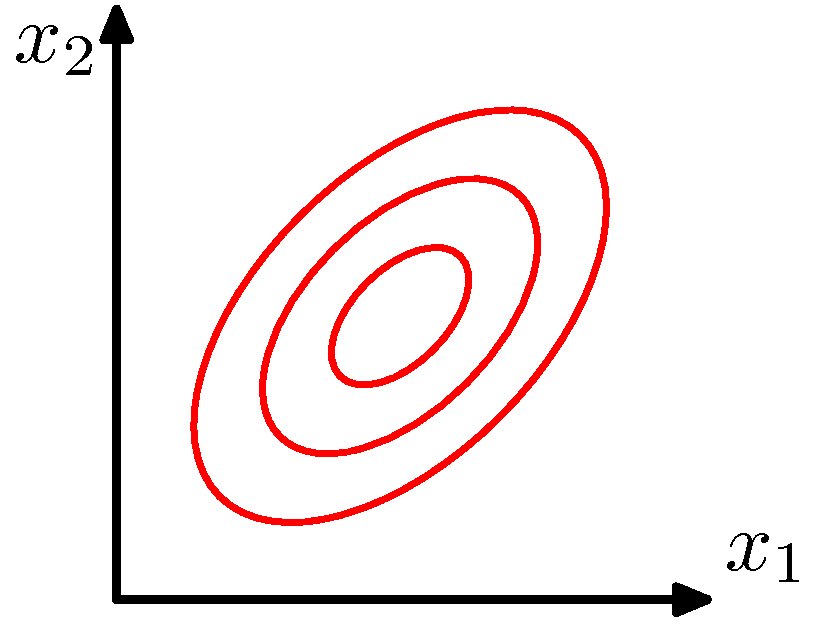
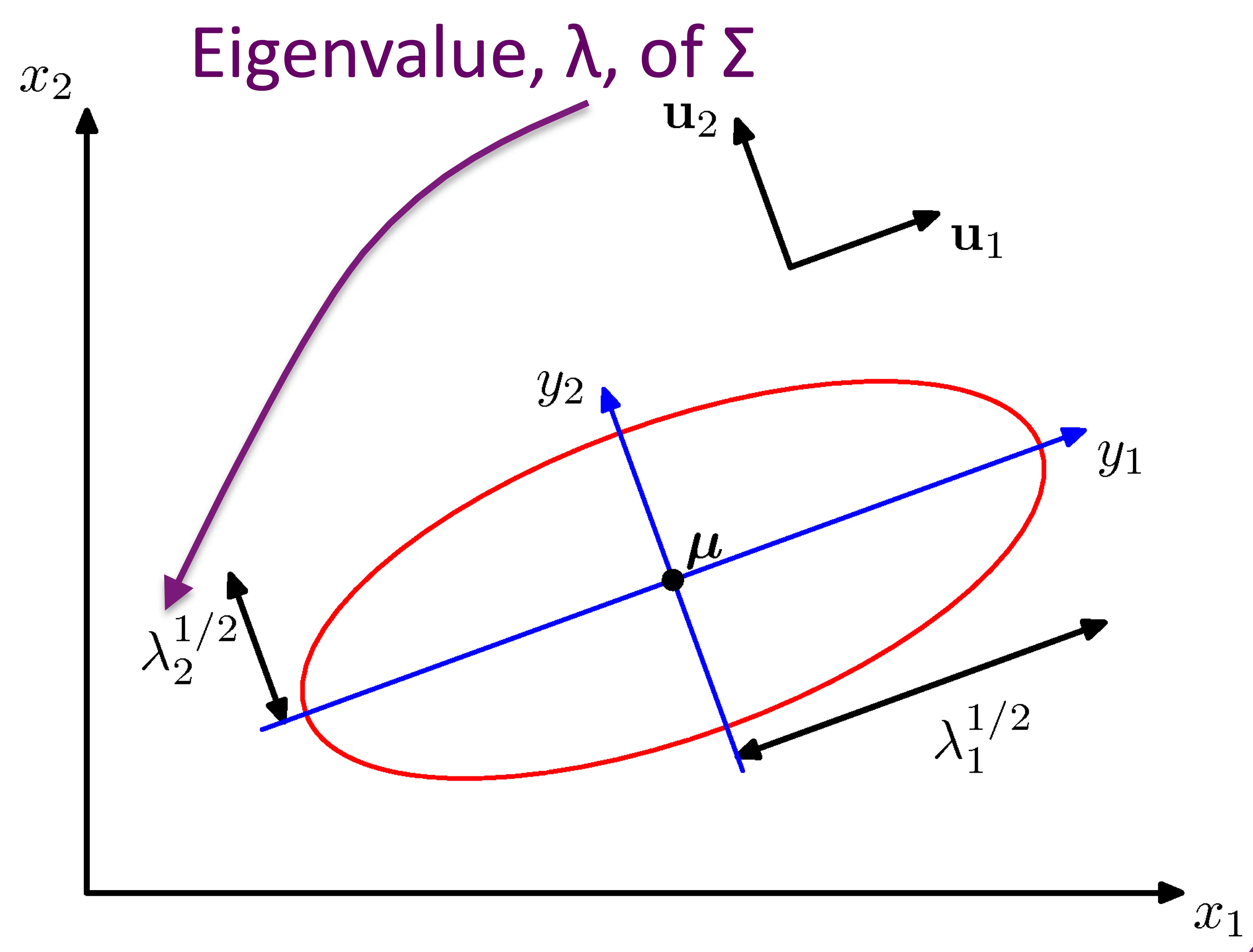
General case
\[P(X=\mathbf{x}_j) = \frac{1}{(2\pi)^{m/2} \|\Sigma\|^{1/2}} \exp\left[-\frac{1}{2}(\mathbf{x}_j - \boldsymbol{\mu})^T \Sigma^{-1} (\mathbf{x}_j - \boldsymbol{\mu})\right]\]
\(\Sigma\) is an arbitrary (semidefinite) matrix
Specifies rotation/change of basis
Eigenvalues specify the relative elongation
\(\Sigma\) accounts for degree to which points vary together
\[P(X=\mathbf{x}_j) = \frac{1}{(2\pi)^{m/2} \|\Sigma\|^{1/2}} \exp\left[-\frac{1}{2}(\mathbf{x}_j - \boldsymbol{\mu})^T \Sigma^{-1} (\mathbf{x}_j - \boldsymbol{\mu})\right]\]
![Visual representation of how the covariance matrix determines the shape and orientation of the Gaussian distribution.]()
How can we even more flexibly fit distributions?
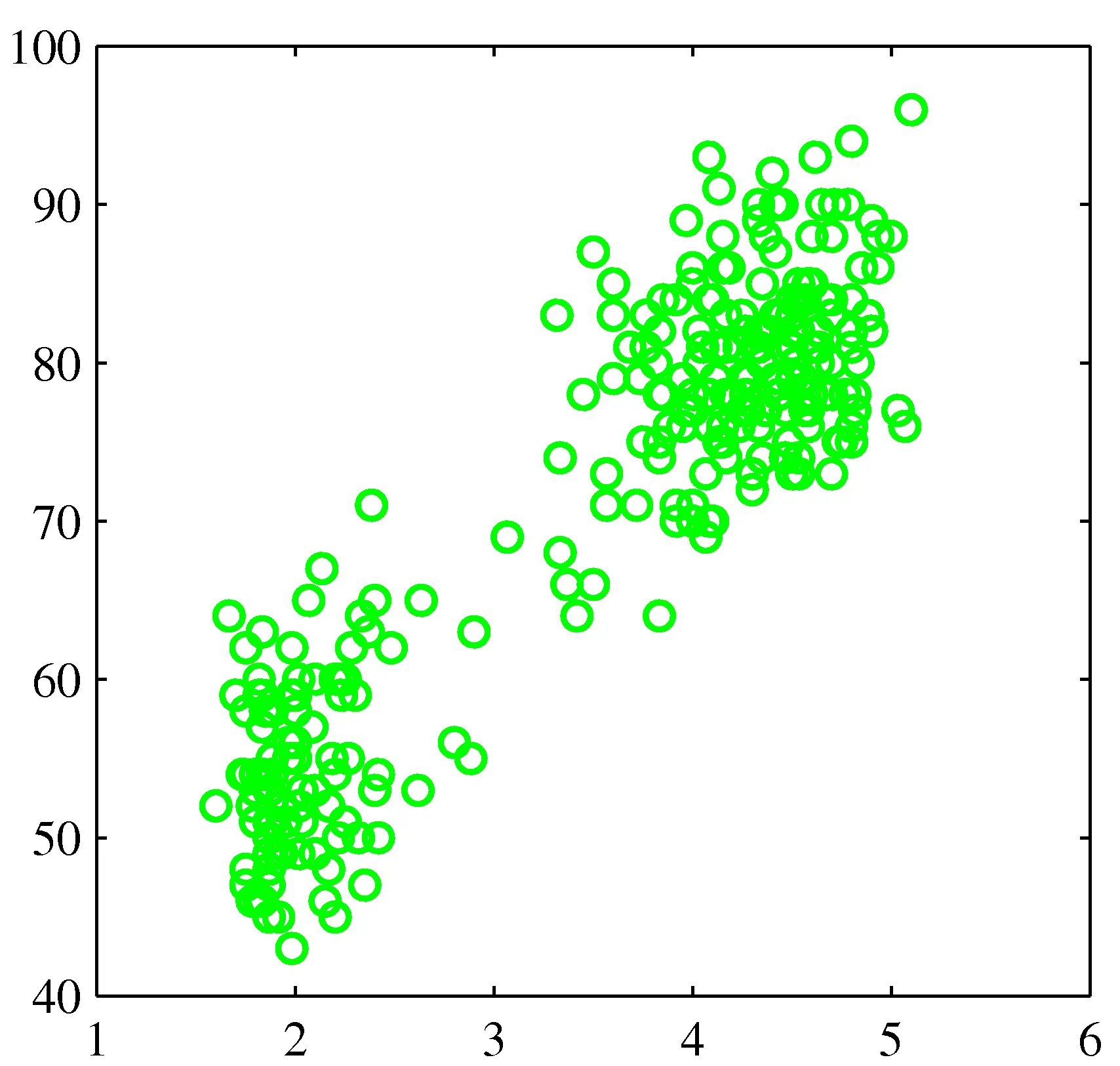
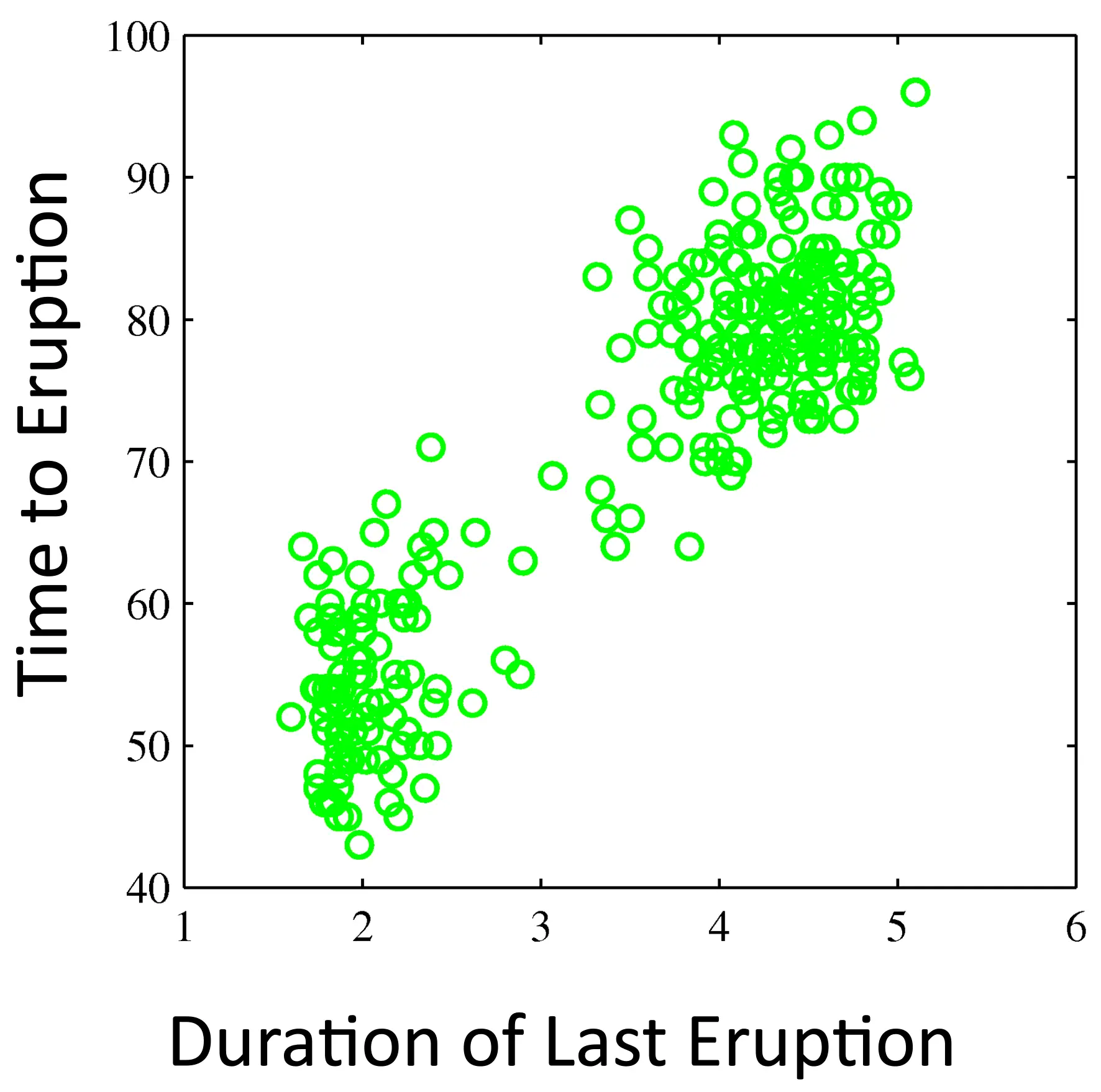
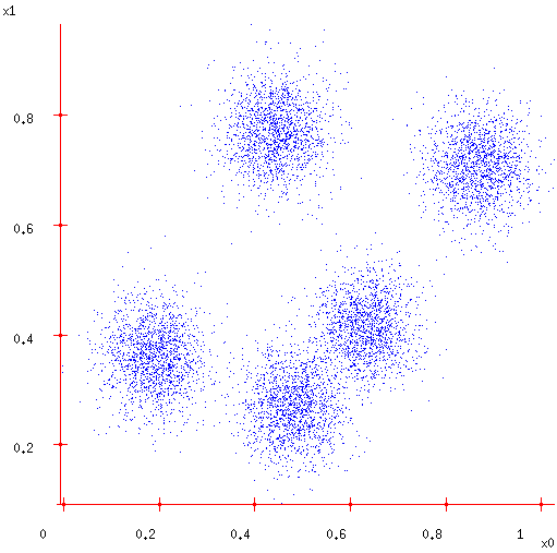
Old Faithful Data Set
![Histogram or scatter plot of the Old Faithful dataset showing two distinct clusters.]()
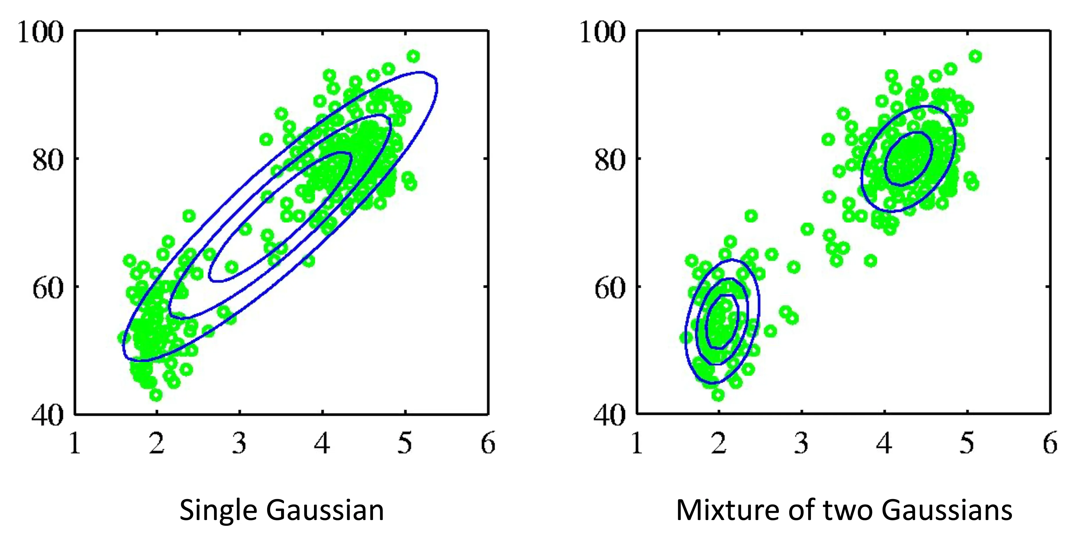
Two distributions might fit the data better
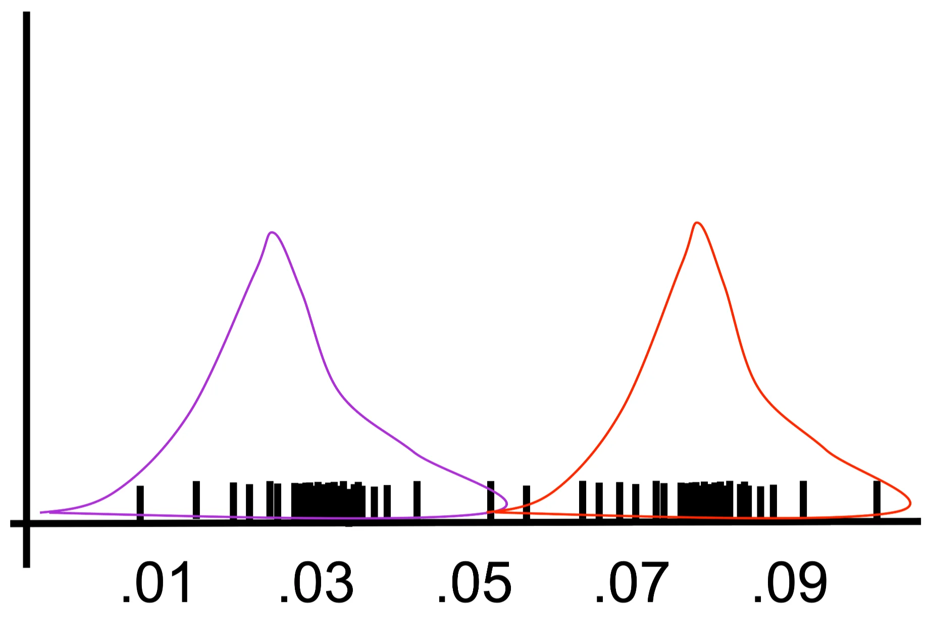
Old Faithful Data Set
![Old Faithful dataset with two Gaussian distributions superimposed, fitting the two modes of the data.]()
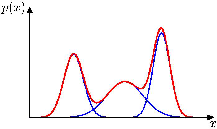
We can make mixtures of distributions!
Combine simple models into a complex model:
\[p(\mathbf{x}) = \sum_{k=1}^K \pi_k \mathcal{N} (\mathbf{x} | \boldsymbol{\mu}_k, \mathbf{\Sigma}_k)\]
\[\forall k: \pi_k \geq 0\]
\[\sum_{k=1}^K \pi_k = 1\]
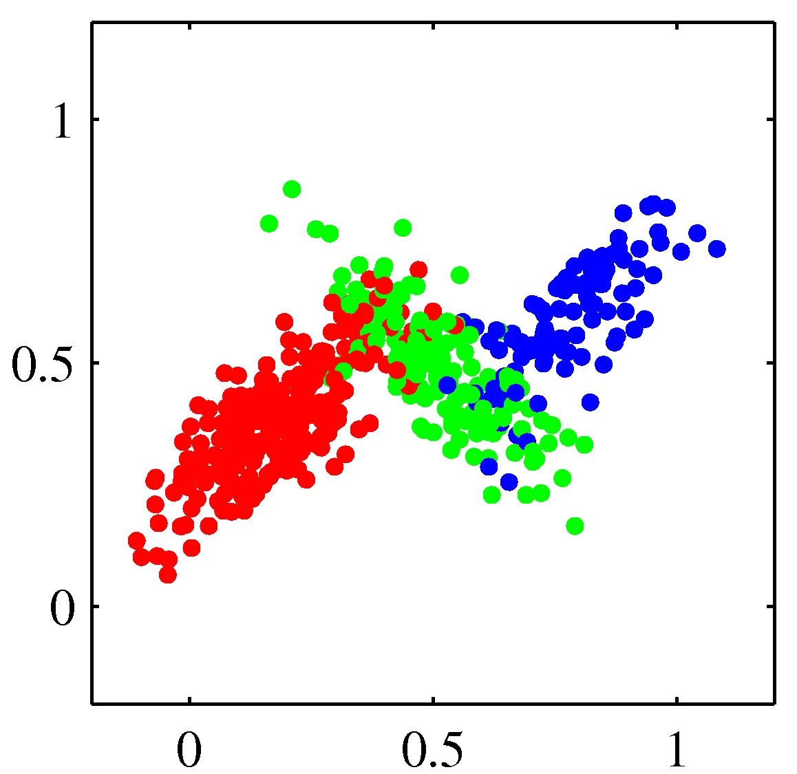
Distribution mixtures eliminate hard assignments
Model data as mixture of multivariate Gaussians
![Visualisation of soft assignments in a Gaussian Mixture Model, where points have probabilities of belonging to each cluster.]()
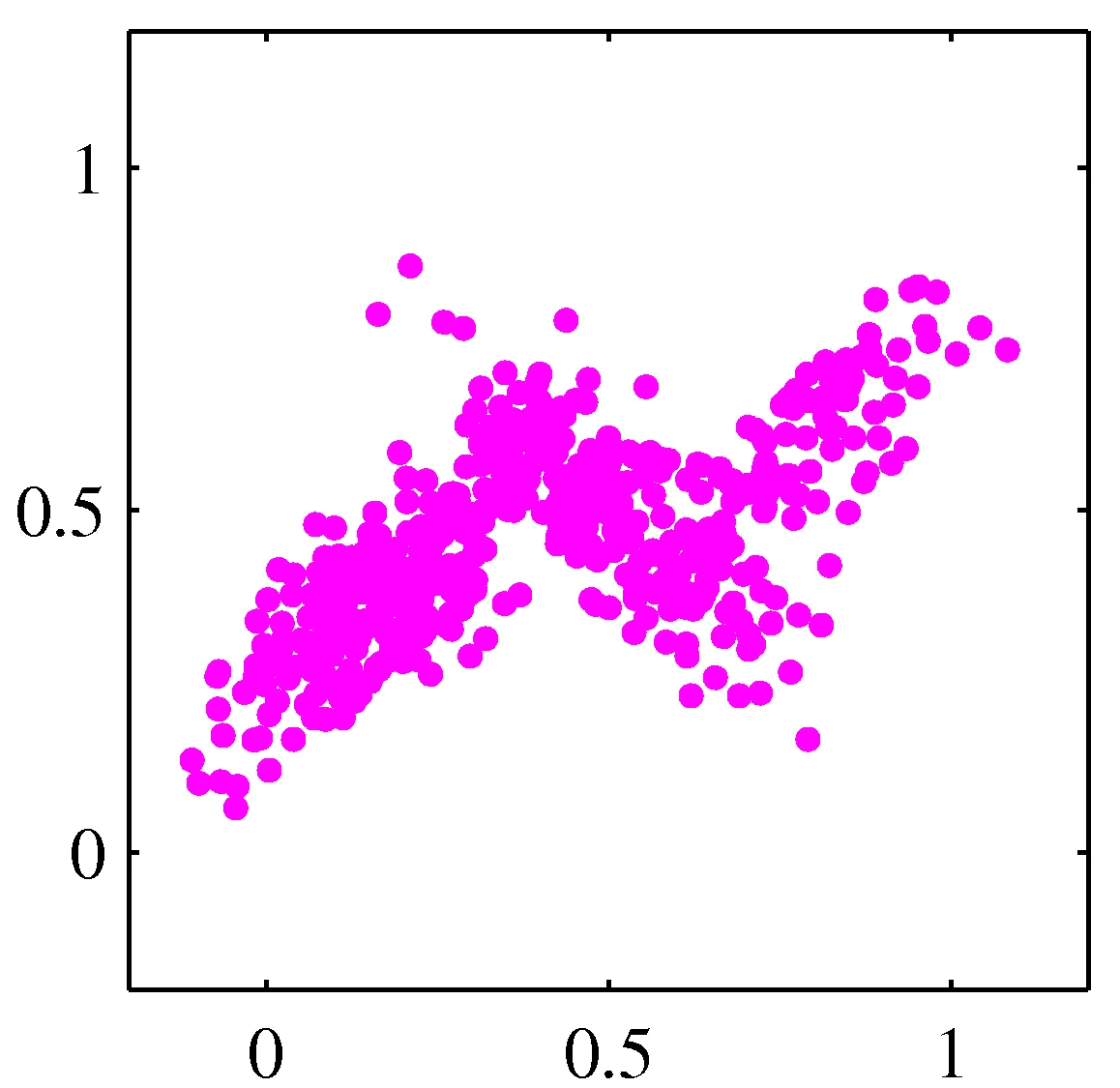
Distribution mixtures eliminate hard assignments
Model data as mixture of multivariate Gaussians
![Another visualization of Gaussian Mixture Model soft assignments.]()
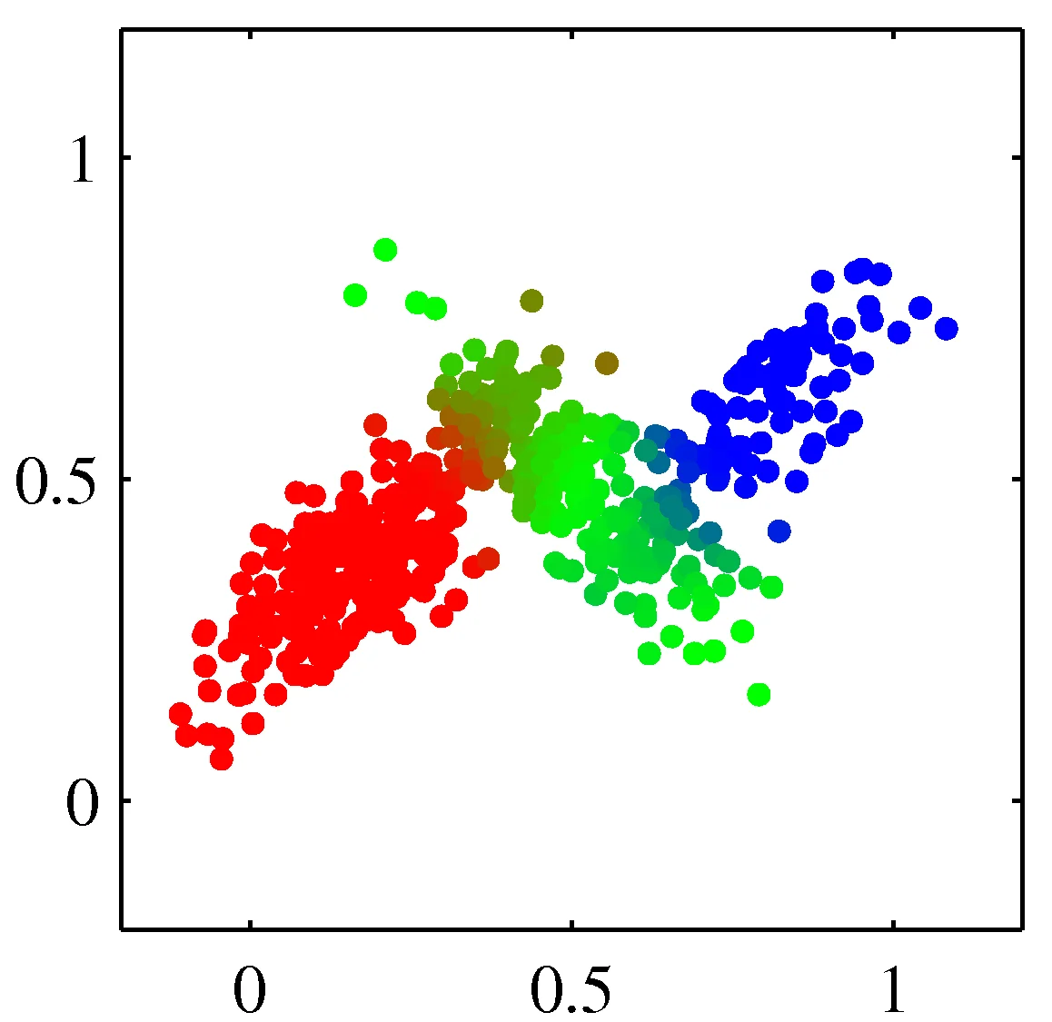
Distribution mixtures eliminate hard assignments
Model data as mixture of multivariate Gaussians
![Plot showing the posterior probability of each data point belonging to a specific Gaussian component.]()
Shown is the posterior probability that a point was generated from \(i\)th Gaussian: \(Pr(Y = i \mid x)\)
Fitting in a supervised setting
Univariate Gaussian
\[\mu_{MLE} = \frac{1}{N}\sum_{i=1}^N x_i \quad\quad \sigma_{MLE}^2 = \frac{1}{N}\sum_{i=1}^N (x_i -\hat{\mu})^2\]
Mixture of Multivariate Gaussians
ML estimate for each of the Multivariate Gaussians is given by:
\[\mu_{ML}^k = \frac{1}{n} \sum_{j=1}^n x_n \quad\quad \Sigma_{ML}^k = \frac{1}{n}\sum_{j=1}^n \left(\mathbf{x}_j - \mu_{ML}^k\right) \left(\mathbf{x}_j - \mu_{ML}^k\right)^T\]
Sums over \(x\) generated from the \(k\)’th Gaussian
But what if unobserved data?
![Diagram representing the concept of unobserved or latent variables in the context of mixture models.]()
But what if unobserved data?
- MLE: \(\arg\max_\theta \prod_j P(y_i, x_j)\)
- \(\theta\): all model parameters
- e.g., class probs, means, and variances
- But we don’t know \(y_j\)’s!
- Maximize marginal likelihood:
- \(\arg\max_\theta \prod_j P(x_j) = \arg\max_\theta \prod_j \sum_{k=1}^K P(Y_j=k, x_j)\)
Learning general mixtures of Gaussians
\[P(y = k | \mathbf{x}_j) \propto \frac{1}{(2\pi)^{n/2} ||\Sigma_k||^{1/2}} \exp\left[-\frac{1}{2}(\mathbf{x}_j - \mu_k)^T \Sigma_k^{-1}(\mathbf{x}_j - \mu_k)\right]P(y = k)\]
Marginal likelihood: \[\prod_{j=1}^m P(\mathbf{x}_j) = \prod_{j=1}^m \sum_{k=1}^K P(\mathbf{x}_j, y = k)\] \[= \prod_{j=1}^m \sum_{k=1}^K \frac{1}{(2\pi)^{n/2} ||\Sigma_k||^{1/2}} \exp\left[-\frac{1}{2}(\mathbf{x}_j - \mu_k)^T \Sigma_k^{-1}(\mathbf{x}_j - \mu_k)\right]P(y = k)\]
Need to differentiate and solve for \(\mu_k\), \(\sum_k\), and P(Y=k) for k=1..K
There will be no closed form solution, gradient is complex, lots of local optimum
Wouldn’t it be nice if there was a better way!?!
General GMMs: Setup
Iterate: On the \(t\)’th iteration let our estimates be
\[ \lambda_t = \{ \mu_1^{(t)}, \mu_2^{(t)} ... \mu_K^{(t)}, \Sigma_1^{(t)}, \Sigma_2^{(t)} ... \Sigma_K^{(t)}, p_1^{(t)}, p_2^{(t)} ... p_K^{(t)} \} \]
\(p_k^{(t)}\) is shorthand for estimate of \(P(y=k)\) on \(t\)’th iteration
General GMMs: E-step
Compute “expected” classes of all datapoints for each class
\[ P(Y_j = k|x_j, \lambda_t) \propto p_k^{(t)}p(x_j|\mu_k^{(t)}, \Sigma_k^{(t)}) \] Just evaluate a Gaussian at \(x_j\)
General GMMs: M-step
Compute weighted MLE for \(\mu\) given expected classes above
\[ \mu_k^{(t+1)} = \frac{\sum_j P(Y_j = k|x_j,\lambda_t)x_j}{\sum_j P(Y_j = k|x_j,\lambda_t)} \]
\[ \Sigma_k^{(t+1)} = \frac{\sum_j P(Y_j = k|x_j,\lambda_t) [x_j - \mu_k^{(t+1)}][x_j - \mu_k^{(t+1)}]^T}{\sum_j P(Y_j = k|x_j,\lambda_t)} \]
\[ p_k^{(t+1)} = \frac{\sum_j P(Y_j = k|x_j,\lambda_t)}{m} \]
\(m\) is the number of training examples
Animation of fitting
![Animation showing the Expectation-Maximization algorithm converging to fit a Gaussian Mixture Model to data.]()
EM for GMMs: only learning means
On the \(t\)’th iteration let our estimates be: \(\lambda_t = \{ \mu_1^{(t)}, \mu_2^{(t)} ... \mu_K^{(t)} \}\)
E-step
Compute “expected” classes of all datapoints
\[P(Y_j = k|x_j, \mu_1 ... \mu_K) \propto \exp(-\frac{1}{2\sigma^2}\|x_j - \mu_k\|^2)P(Y_j = k)\]
M-step
Compute most likely new \(\mu\)s given class expectations
\[\mu_k = \frac{\sum_{j=1}^{m} P(Y_j = k|x_j) x_j}{\sum_{j=1}^{m} P(Y_j = k|x_j)}\]
What if we do hard assignments?
On the \(t\)’th iteration let our estimates be \(\lambda_t = \{ \mu_1^{(t)}, \mu_2^{(t)} ... \mu_K^{(t)} \}\)
E-step
Compute “expected” classes of all datapoints
\[P(Y_j = k | x_j, \mu_1...\mu_K) \propto \exp(-\frac{1}{2\sigma^2}\|x_j - \mu_k\|^2)\]
What if we do hard assignments?
On the t’th iteration let our estimates be \(\lambda_t = \{ \mu_1^{(t)}, \mu_2^{(t)} ... \mu_K^{(t)} \}\)
M-step
Compute most likely new \(\mu\)s given class expectations \[\mu_k = \frac{\sum_{j=1}^m \delta(Y_j=k,x_j)x_j}{\sum_{j=1}^m \delta(Y_j=k,x_j)}\]
\(\delta\) represents hard assignment to “most likely” or nearest cluster
Equivalent to k-means clustering algorithm!
Implementation
sklearn.mixture.GaussianMixture implements GMMs within sklearn.
GaussianMixture creates the class
n_components indicates the number of Gaussians to use.covariance_type is type of covariance
fullsphericaldiagtied means all components share the same covariance matrix
max_iter is EM iterations to use
- Functions
M.fit(X) fits using the EM algorithmM.predict_proba(X) is the posterior probability of each component given the dataM.predict(X) predict the class labels of each data point