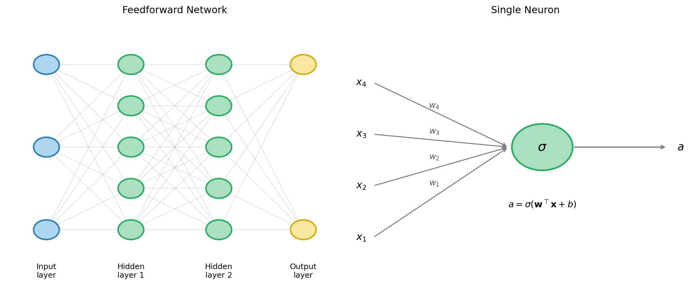
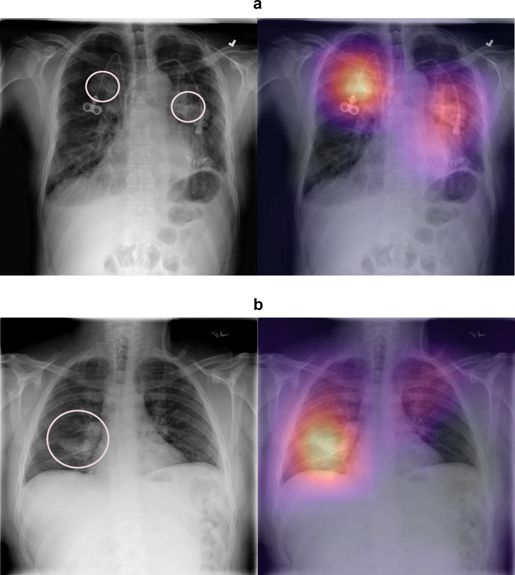
Neural Networks

Aaron Meyer

Outline

• Neural Network Architecture
• Backpropagation
• Regularization in Neural Networks
• Structure as Inductive Bias
• Applications in Bioengineering
• Review

Why can’t simpler models handle this?

• The feature space is high-dimensional: images + mechanical signals
• The relevant structure is nonlinear: cell type isn’t linearly separable in raw pixel space
• The “right” features are unknown a priori: handcrafted features miss what matters
• Neural networks learn a hierarchy of features directly from the data

Contrast with logistic regression (linear decision boundary), PCA (linear structure), and even regularized regression. Each of those requires the right features to already exist. Neural networks discover the features themselves.

Neural Network Architecture

From Neurons to Networks

• A single artificial neuron computes: \[a = \sigma\left(\sum_{i} w_i x_i + b\right) = \sigma(\mathbf{w}^\top \mathbf{x} + b)\]
  • \(\mathbf{x}\): inputs; \(\mathbf{w}\): weights; \(b\): bias; \(\sigma\): activation function
• A layer applies this operation to every neuron in parallel
• A network stacks multiple layers: the output of one layer is the input to the next

The key is the nonlinear activation function σ. Without it, stacking layers would just be matrix multiplication—equivalent to a single linear layer. The nonlinearity is what allows deep networks to represent complex functions.

Feedforward network architecture

A fully connected feedforward network. Each node computes a weighted sum of its inputs, then applies an activation function.

Activation Functions

Common activation functions. ReLU dominates modern hidden layers; sigmoid and softmax are used in output layers for classification.

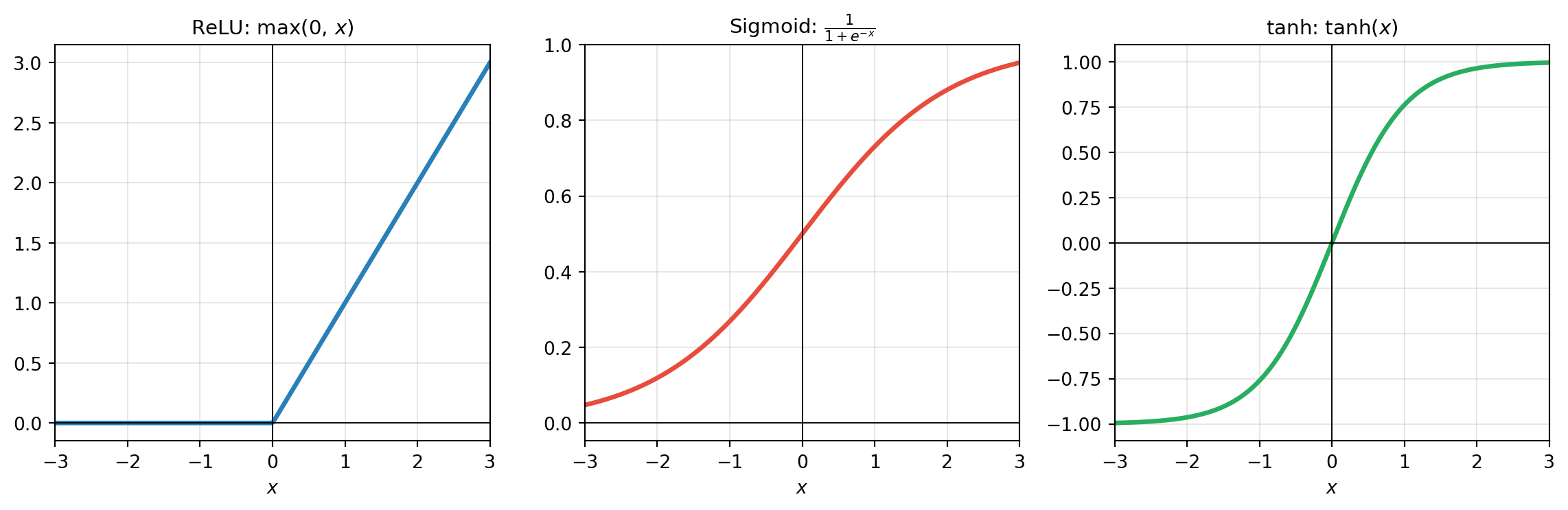
• ReLU (rectified linear unit): sparse, fast to compute, avoids vanishing gradient—the default choice for hidden layers
• Sigmoid: output in \((0,1)\)—useful for binary probability outputs
• tanh: output in \((-1,1)\)—zero-centered, often used in recurrent networks

The choice of activation function matters a lot in practice. ReLU and its variants (leaky ReLU, GELU) dominate modern architectures. The key property is that the derivative is non-zero in at least some region—this allows gradients to flow during training.

Backpropagation

Backprop Is Reverse-Mode Autodiff

• Recall from the autodifferentiation lecture:
  • Reverse mode: one forward pass + one backward pass computes the gradient w.r.t. all parameters in \(O(1)\) function evaluations
  • Cost ∝ cost of the forward pass, regardless of parameter number
• Backpropagation is exactly reverse-mode autodiff applied to a neural network: \[\frac{\partial L}{\partial w_{ij}^{(\ell)}} = \frac{\partial L}{\partial a_j^{(\ell)}} \cdot \frac{\partial a_j^{(\ell)}}{\partial z_j^{(\ell)}} \cdot \frac{\partial z_j^{(\ell)}}{\partial w_{ij}^{(\ell)}}\] where \(z_j^{(\ell)} = \mathbf{w}_j^{(\ell)\top}\mathbf{a}^{(\ell-1)} + b_j^{(\ell)}\) and \(a_j^{(\ell)} = \sigma(z_j^{(\ell)})\)

This is the chain rule, applied layer by layer, moving backwards through the network. The “delta” terms are the error signals propagated from the output. Modern frameworks (PyTorch, JAX, TensorFlow) implement this automatically—you never write backprop by hand.

The connection to autodiff is important: backprop is not a special algorithm unique to neural networks. It is a special case of reverse-mode AD applied to a specific computational graph. JAX’s jax.grad computes this for any function, not just neural networks.

Training loop in practice

import jax
import jax.numpy as jnp
import optax  # gradient-based optimizers

# Define network forward pass
def predict(params, x):
    for W, b in params[:-1]:
        x = jax.nn.relu(x @ W + b)
    W, b = params[-1]
    return x @ W + b

# Loss function
def loss_fn(params, x_batch, y_batch):
    preds = predict(params, x_batch)
    return jnp.mean((preds - y_batch) ** 2)

# Gradient via reverse-mode autodiff
grad_fn = jax.jit(jax.grad(loss_fn))

# Stochastic gradient descent step
optimizer = optax.adam(learning_rate=1e-3)
opt_state = optimizer.init(params)

for x_batch, y_batch in dataloader:
    grads = grad_fn(params, x_batch, y_batch)
    updates, opt_state = optimizer.update(grads, opt_state)
    params = optax.apply_updates(params, updates)

Point out that jax.grad does all the backpropagation automatically. The user just specifies the forward pass and the loss. The training loop is: compute gradient, update parameters, repeat. Mini-batching (not the full dataset each step) makes this tractable for large datasets.

The non-convex optimization landscape

• Unlike ridge regression or LASSO, the neural network loss surface is non-convex

  • Multiple local minima exist
  • The landscape has saddle points and flat regions (“plateaus”)

• Classical convex optimization guarantees do not apply

• Yet in practice, large overparameterized networks train reliably. Why?

  • In very high dimensions, local minima tend to have similar loss values
  • Stochastic gradient descent (SGD) acts as an implicit regularizer—it finds “flat” minima that generalize better than sharp ones

This is an active research area. The key empirical observation is that for sufficiently overparameterized models, the loss landscape has very few “bad” local minima. Most local minima are near the global minimum. This is not true for small networks.

The SGD implicit bias toward flat minima is related to the double descent story: SGD finds solutions that are “smooth” in weight space, which tends to generalize well.

Regularization in Neural Networks

The Gap Between Theory and Practice

• The Universal Approximation Theorem guarantees that a large enough network can represent the target function
• But in practice, without regularization:
  • Large networks memorize noise
  • Training diverges or oscillates
  • Generalization fails badly
• Everything we know about regularization still applies, just adapted to the NN setting

Stop here, ask for ways of making overparameterized networks generalize.

This is the key message of this section. Double descent and UAT explain why overparameterized networks can generalize, but they don’t tell you how to make them generalize in practice. That requires the techniques in this section.

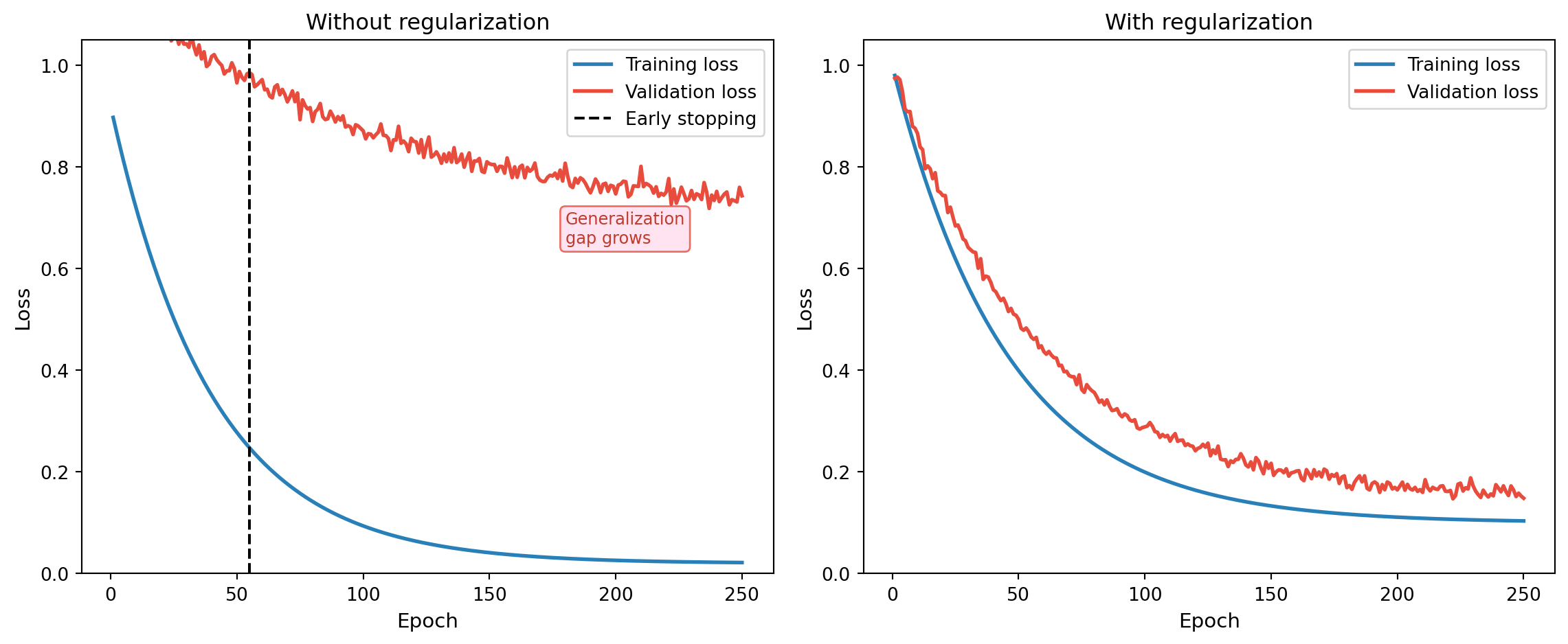
Training curves without and with regularization

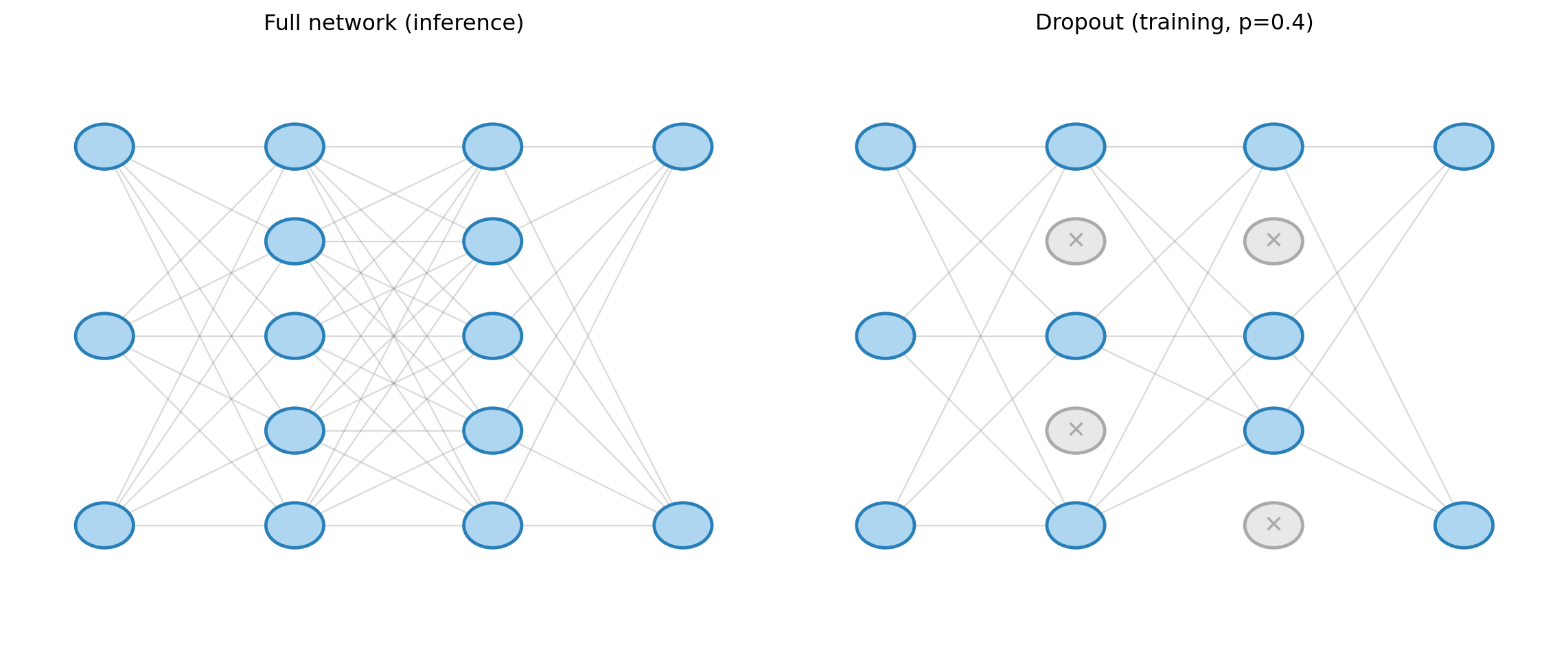
Training and validation loss with and without regularization. Without regularization, the network memorizes training data but fails to generalize. Early stopping (dashed line) is a simple regularizer.

Weight Decay

• Weight decay adds an \(\ell_2\) penalty to the loss—directly analogous to ridge regression: \[L_\text{reg}(\boldsymbol{\theta}) = L(\boldsymbol{\theta}) + \frac{\lambda}{2}\|\boldsymbol{\theta}\|_2^2\]
• Penalizes large weights; shrinks them toward zero during training
• Bayesian interpretation: Gaussian prior \(\theta_j \sim \mathcal{N}(0, 1/\lambda)\) on each weight
  • From the Bayesian lecture: MAP estimation with a Gaussian prior = \(\ell_2\) regularization

This is a direct callback to both the regularization lecture (ridge regression) and the Bayesian lecture (MAP = regularization). The same principle works at scale.

Note: in neural networks, we typically don’t regularize bias terms—only weights.

Dropout

• During each forward pass, randomly zero out a fraction \(p\) of neurons (Srivastava et al., 2014)
• At test time, scale all activations by \((1-p)\) to preserve expected magnitude

Dropout at training time: a random subset of neurons is silenced each forward pass. This forces the network to learn redundant representations.

Dropout forces the network to learn distributed representations: no single neuron can “specialize” and be relied upon because it might be dropped. At test time, the full network is used but with scaled activations—this approximates averaging over the exponentially many thinned networks, which is an ensemble method.

Dropout can also be interpreted as approximate Bayesian inference (Gal & Ghahramani, 2016)—connecting again to the Bayesian lecture.

Batch normalization

• After each layer, normalize activations to have zero mean and unit variance across the training mini-batch: \[\hat{x}_i = \frac{x_i - \mu_\mathcal{B}}{\sqrt{\sigma_\mathcal{B}^2 + \epsilon}}, \qquad y_i = \gamma \hat{x}_i + \delta\]
• Learnable scale \(\gamma\) and shift \(\delta\) restore representational capacity
• Benefits:
  • Stabilizes optimization: prevents activations from exploding or vanishing
  • Acts as mild regularization (adding noise through batch statistics)
  • Allows higher learning rates → faster training

Batch norm was introduced by Ioffe & Szegedy (2015) and became ubiquitous quickly. The mechanism is still debated—it was originally motivated as reducing “internal covariate shift,” but later work showed the optimization stability benefit is the dominant effect.

Summary: regularization toolkit for neural networks

Method	Mechanism	Analogy
Weight decay	\(\ell_2\) penalty on weights	Ridge regression
Dropout	Random neuron silencing	Ensemble averaging
Early stopping	Stop before validation loss rises	Cross-validation
Batch norm	Normalize activations per batch	Conditioning
Data augmentation	Random transforms of training data	Effectively enlarges \(n\)

In practice, you use all of these simultaneously. The specific strengths depend on the architecture and dataset. Data augmentation (not shown in detail) is often the most powerful: for images, random flips/crops/color jitter; for molecules, random rotations; for sequences, random masking.

Structure as Inductive Bias

The Key Insight

• A fully connected network is structure-agnostic: it treats all inputs symmetrically
• This is flexible, but expensive: it must learn from scratch that nearby pixels are correlated, that molecules are rotation-invariant, that sequences have order
• Inductive biases bake known structure into the architecture:
  • Less data needed to learn the relevant function
  • Better generalization on finite datasets
  • Often leads to models that are interpretable in domain terms

This is the deepest conceptual point of the lecture. UAT says any function is representable; inductive biases say which function is easy to learn. The history of deep learning is largely a history of discovering the right inductive biases for each domain.

Inductive biases are another form of regularization—they constrain the hypothesis space to functions consistent with our domain knowledge.

Convolutional Neural Networks (CNNs)

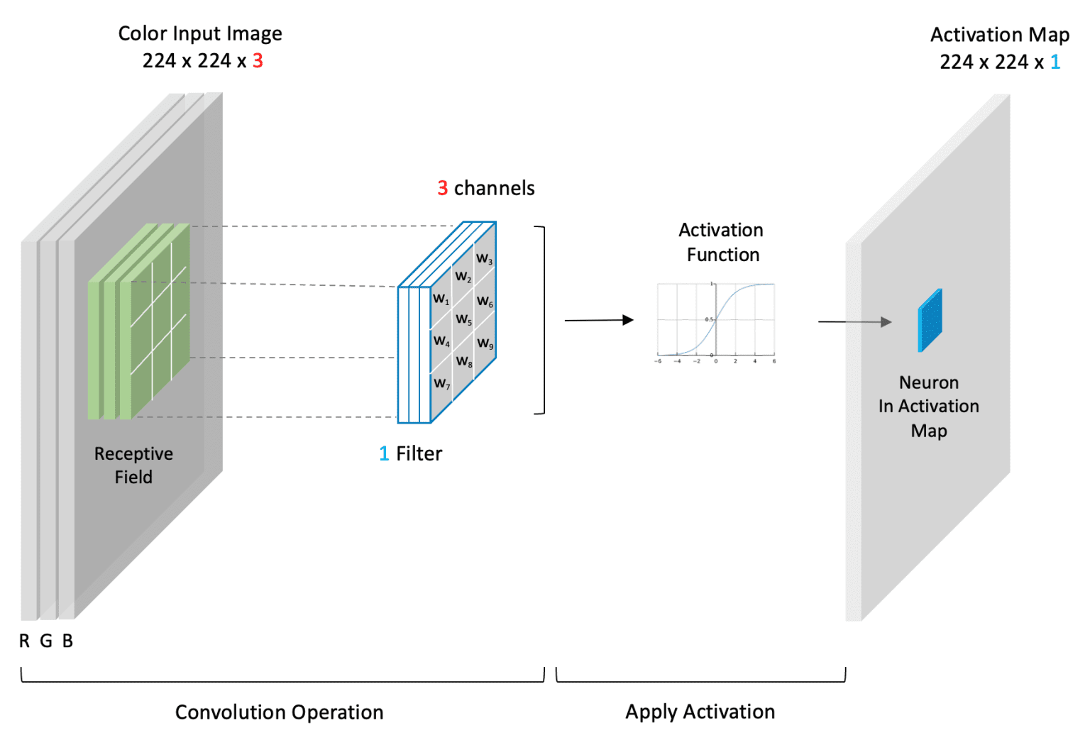
• Designed for spatially structured data (images, 1-D signals)
• Two key inductive biases:
  1. Local connectivity: neurons connect only to nearby inputs—nearby pixels are more related
  2. Weight sharing: the same filter is applied across all spatial positions (translation equivariance)

\[(\mathbf{W} * \mathbf{x})_{i,j} = \sum_{k,\ell} W_{k,\ell} \cdot x_{i+k,\, j+\ell}\]

• Many fewer parameters than fully connected layers for image-sized inputs
• Applications in biology: cell morphology, histology, microscopy image analysis

For many images, translation equivariance is exactly right: a cell in the top-left corner should be classified the same way as the same cell in the bottom-right corner.

Note: convolutional layers are not the same as Fourier transforms, but they share the translation equivariance property.

Graph Neural Networks (GNNs)

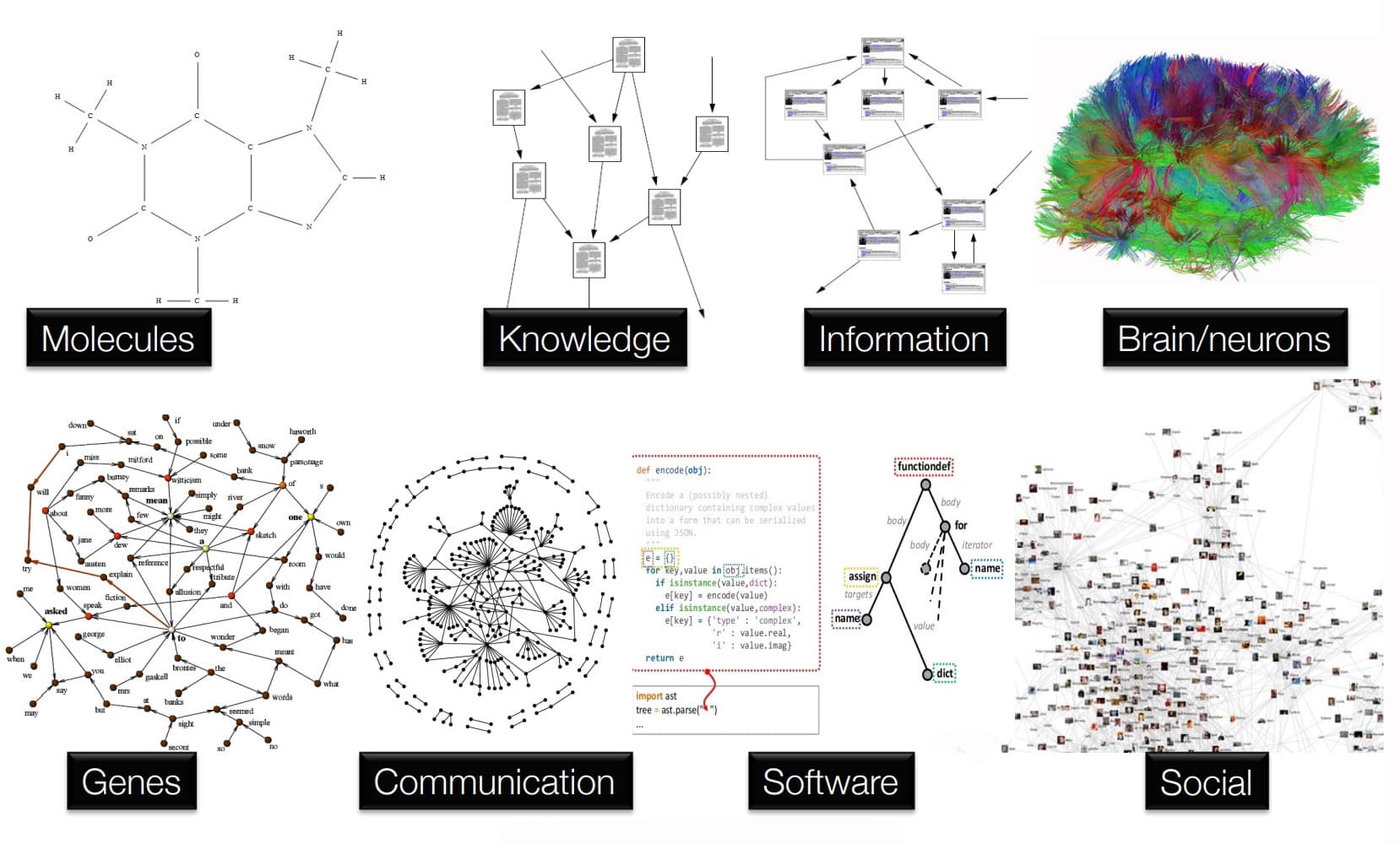
• Designed for data with relational structure (graphs, molecules, interaction networks)
• Update node features by aggregating information from neighbors: \[\mathbf{h}_v^{(\ell+1)} = \sigma\left(\mathbf{W}^{(\ell)} \cdot \text{AGGREGATE}\left(\left\{\mathbf{h}_u^{(\ell)} : u \in \mathcal{N}(v)\right\}\right)\right)\]
• Key inductive biases:
  • Permutation invariance over the node set (molecules have no canonical atom ordering)
  • Local neighborhood aggregation reflects chemical bonding
• Applications in bioengineering:
  • Drug-target interaction prediction
  • Protein–protein interaction networks
  • Metabolic pathway modeling

GNNs are arguably the most important architecture for bioengineering applications because biology is fundamentally a graph-structured discipline: signaling networks, metabolic networks, protein contact maps. The structure of the graph reflects causal relationships, and GNNs can exploit this.

Attention and Transformers

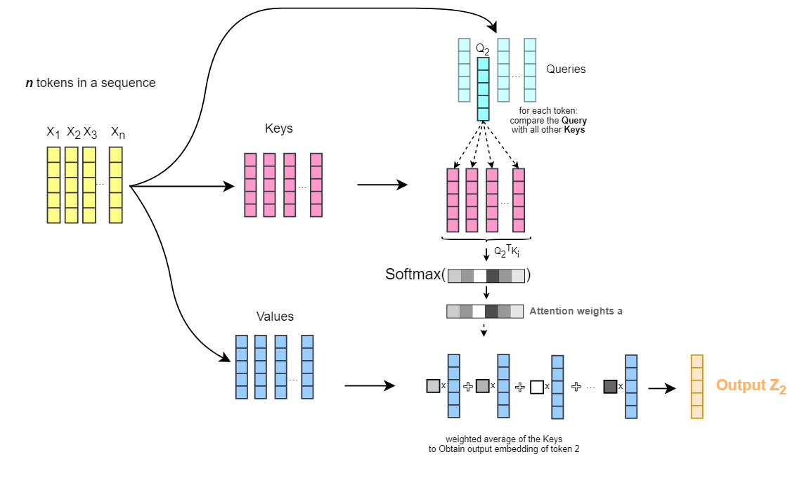
• Rather than fixed local connectivity, attention learns which inputs to weight: \[\text{Attention}(Q, K, V) = \text{softmax}\left(\frac{QK^\top}{\sqrt{d_k}}\right) V\]

• Inductive bias: relational structure is data-dependent, not hardcoded

• More flexible than CNNs and GNNs—but requires more data to learn useful structure

• Bioengineering applications:

  • Protein language models (ESM, ProtTrans): treat protein sequence like text
  • AlphaFold2: combines attention over sequence + structural inductive biases
  • Single-cell transformers: model gene expression programs

The transformer architecture (Vaswani et al., 2017) was developed for NLP but has since dominated biology. The key insight is that “attention” generalizes to any domain where pairwise relationships matter. AlphaFold2 uses attention over both sequence and predicted pair representations. The inductive biases are about protein geometry (residue distance, angles), not just sequence order.

Applications in Bioengineering

Drug Response Prediction (Revisited)

• In the regularization lecture, we used elastic net to predict drug sensitivity from genomic features in the CCLE
• Neural networks can capture nonlinear gene–drug interactions
• With enough data, a deep network often outperforms LASSO/ridge
• But: neural networks require more data and careful regularization
• With 500 cell lines, regularized linear models often win

This is an important practical lesson. Neural networks are not automatically better than simpler models. For n=500, the extra capacity of a deep network often leads to overfitting unless extremely well-regularized. The tradeoff shifts as n increases; this is another manifestation of double descent.

Protein structure prediction: AlphaFold2

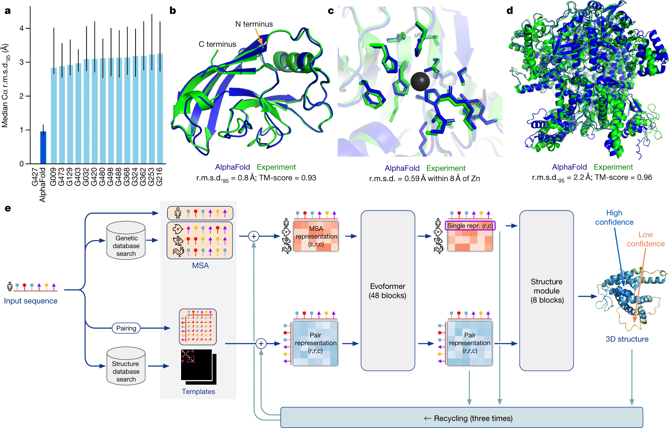
• Why it works: massive structural inductive bias
  • Equivariance to rotation and translation of the protein backbone
  • Pair representation explicitly encodes residue–residue distances
  • Iterative “recycling” refines structure over multiple passes
• Training data: ~170,000 experimentally solved structures (PDB)
• Result: Near-experimental accuracy on most proteins
• Solved a 50-year-old problem

AlphaFold is the most striking example of what the right inductive biases can achieve. The network has ~93M parameters trained on ~170K structures—roughly 550 parameters per training example. This is highly regularized by bioengineering standards. The key was not just scale, but the right structural biases: triangular attention, equivariant frames, and evolutionary covariation signal.

Jumper et al., Nature 2021.

Cell morphology as a phenotypic readout

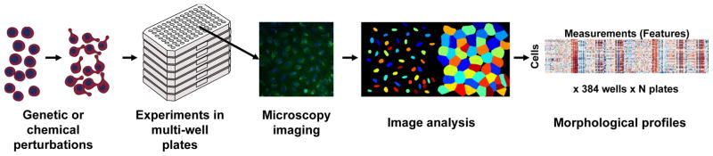
• Cell Painting (Bray et al., 2016): image cells stained with 6 fluorescent dyes; extract ~1,500 morphological features
• Neural networks trained on raw images learn features that correlate with:
  • Mechanism of action of compounds
  • Disease phenotype
  • Genetic perturbation identity
• Architecture: CNN backbone (treats image as spatially structured) + classification head

This connects directly to the Masaeli et al. paper. The key insight is that cell morphology is a rich, high-dimensional phenotype that encodes biological state. Neural networks, especially with CNN inductive biases, can extract this information in ways that hand-crafted features cannot.

Review

Further Reading

• LeCun Y., Bengio Y., Hinton G. Deep learning. Nature, 2015.
• Srivastava N. et al. Dropout: A Simple Way to Prevent Neural Networks from Overfitting. JMLR, 2014.
• Jumper J. et al. Highly accurate protein structure prediction with AlphaFold. Nature, 2021.
• Ching T. et al. Opportunities and obstacles for deep learning in biology and medicine. J. R. Soc. Interface, 2018.
• Masaeli M. et al. Multicolor fluorescence imaging to study cell heterogeneity. Sci. Rep., 2016.
• sklearn: Neural network models

Review Questions

1. What is the role of the activation function in a neural network? What would happen if all activations were linear?
2. Explain how backpropagation is a special case of reverse-mode autodifferentiation. What is computed in the forward pass, and what is computed in the backward pass?
3. Why is the neural network loss surface non-convex? What practical consequences does this have for training?
4. A colleague trains a network and observes that training loss continues to decrease while validation loss starts to rise. What is happening, and what would you do?
5. What is an inductive bias? Give one example from each of: CNNs, GNNs, and attention mechanisms, and explain what assumption about the data each encodes.
6. A fully connected network and a CNN are each trained on the same image classification task. The CNN uses far fewer parameters. Under what conditions might the simpler CNN outperform the larger fully connected network?
7. AlphaFold2 has ~93M parameters trained on ~170K examples. How do you reconcile this with the double descent picture—shouldn’t such an overparameterized model need far more data?