Double Descent and the Overparameterization Paradox

Aaron Meyer

Outline

• Application
• The Classical Bias-Variance Picture
• The Interpolation Threshold
• Double Descent
• Universal Approximation
• Review

Application

Predicting Binding at Equilibrium

• A ligand \(L\) binds a receptor \(R\) to form a complex \(RL\): \[R + L \underset{k_\text{off}}{\stackrel{k_\text{on}}{\rightleftharpoons}} RL\]
• At equilibrium, the dissociation constant is: \[K_d = \frac{k_\text{off}}{k_\text{on}} = \frac{[R][L]}{[RL]}\]
• Fractional occupancy follows the saturation isotherm: \[\theta = \frac{[L]}{K_d + [L]}\]

Remind students this is the Hill equation with n=1 (no cooperativity). We want to motivate that a two-parameter system has a deep degeneracy that turns out not to matter for prediction.

What can we learn from equilibrium binding data?

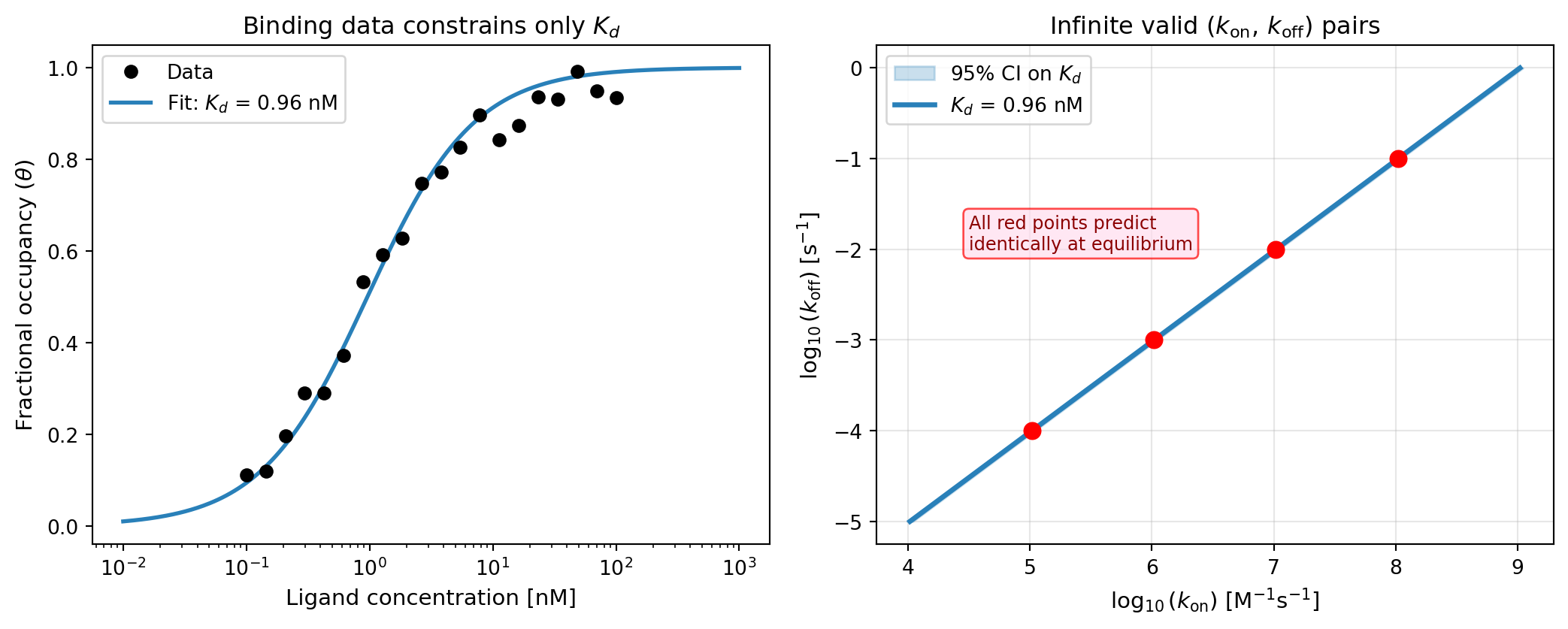
• Measuring \(\theta\) vs. \([L]\) gives us a binding curve
• Fitting the curve estimates \(K_d\), but not \(k_\text{on}\) or \(k_\text{off}\) individually
• Infinitely many \((k_\text{on}, k_\text{off})\) pairs are consistent with any measured \(K_d\): \[k_\text{off} = K_d \cdot k_\text{on} \quad \Rightarrow \quad \text{a 1-D manifold in parameter space}\]
• Yet every point on this manifold makes identical equilibrium predictions

This is the core paradox: we have a model with two free parameters (k_on, k_off), but only a one-dimensional combination of them is constrained by our data. The system is underdetermined. Yet we can still predict perfectly.

Ask students: does this mean the model is “bad” because it’s underdetermined? No—the structure of the prediction problem means only Kd matters. This is the key intuition we’ll generalize.

Left: binding data fit by a single Kd. Right: the infinite manifold of (k_on, k_off) pairs consistent with the data—all make identical equilibrium predictions.

Walk through both panels. The binding curve on the left looks like a clean sigmoid—we fit Kd easily. The right panel shows that Kd constrains a line in parameter space. The red dots are four different models that are biologically indistinguishable at equilibrium.

Key message: underdetermined parameter space does not prevent accurate predictions. We will see this theme recur in machine learning.

The Classical Bias-Variance Picture

Review: Prediction Error Decomposition

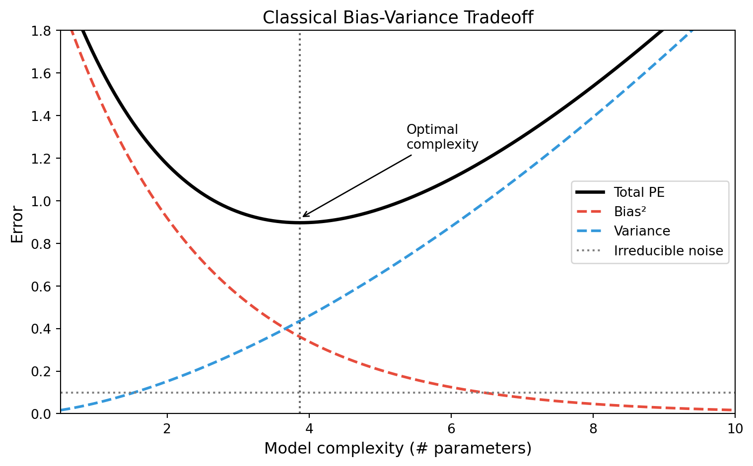
\[\mathrm{PE}(\mathbf{z}_0) = \sigma_\epsilon^2 + \mathrm{Bias}^2\!\left(\hat{f}(\mathbf{z}_0)\right) + \mathrm{Var}\!\left(\hat{f}(\mathbf{z}_0)\right)\]

• Bias: systematic error—does our model class contain the true function?
• Variance: sensitivity to which training samples we happened to draw
• Classical advice: choose model complexity to trade off bias against variance

The Classical U-Curve

Classical bias-variance tradeoff: an optimal complexity minimizes total test error. Regularization (dashed) shifts the optimum.

This is a review from the regularization lecture. The key message is that classical theory says there is a sweet spot, and going beyond it (adding more parameters) increases variance and worsens generalization. This is the intuition we’re about to challenge.

What does classical theory predict for very large models?

• As \(p \to \infty\) (more parameters than data points \(n\)), the model can fit the training data exactly
• This is called interpolation: training error \(\to 0\)
• Classical wisdom: interpolating models overfit catastrophically
  • Variance \(\to \infty\) at the interpolation threshold
  • Prediction error should blow up

Question: Is this always true?

Ask students to think about what “fitting the training data exactly” means for prediction. Classical linear algebra says an underdetermined system has infinitely many solutions—and the least squares solution could be wildly oscillatory. But does it have to be?

This sets up the punchline: no, it doesn’t, and the reason connects back to the binding example.

The Interpolation Threshold

When \(p = n\): Exact Determination

• With exactly \(p = n\) parameters and full-rank design matrix, there is a unique solution that interpolates the data
• This solution can have very large coefficients—high variance
• Test error peaks here: the model has just enough freedom to memorize noise

When \(p > n\): Underdetermined Systems

• Infinitely many parameter vectors \(\hat{\boldsymbol{\theta}}\) satisfy \(\mathbf{X}\hat{\boldsymbol{\theta}} = \mathbf{y}\)
• Standard solvers (e.g., numpy.linalg.lstsq) return the minimum-norm solution: \[\hat{\boldsymbol{\theta}}^+ = \mathbf{X}^\top (\mathbf{X}\mathbf{X}^\top)^{-1} \mathbf{y}\]
• Among all interpolating solutions, this is the one with smallest \(\|\boldsymbol{\theta}\|_2\)

This is the Moore-Penrose pseudoinverse solution. It is analogous to ridge regression in the limit λ → 0. In practice, gradient descent on overparameterized linear models also converges to this minimum-norm solution when initialized at zero.

Connection to the binding example

• Recall: from binding data, the data constrains \(K_d = k_\text{off}/k_\text{on}\), a 1-D subspace of 2-D parameter space
• The minimum-norm solution picks the shortest vector in this subspace: physically, the point where \(k_\text{on}\) and \(k_\text{off}\) are both smallest
• But all solutions make the same equilibrium predictions

Analogy	Binding	Machine Learning
Parameters	\((k_\text{on}, k_\text{off})\)	Weights \(\boldsymbol{\theta}\)
Constraint	\(k_\text{off}/k_\text{on} = K_d\)	\(\mathbf{X}\boldsymbol{\theta} = \mathbf{y}\)
Prediction	\(\theta = [L]/(K_d + [L])\)	\(\hat{y} = \mathbf{x}^\top \boldsymbol{\theta}\)
Solution space	1-D manifold	Affine subspace

This is the conceptual key. In both cases: 1. The data is insufficient to determine all parameters individually. 2. Only a lower-dimensional combination matters for prediction. 3. The minimum-norm solution generalizes well because it is “smooth”—it doesn’t put unnecessary structure in directions not constrained by data.

Double Descent

Extending the Risk Curve

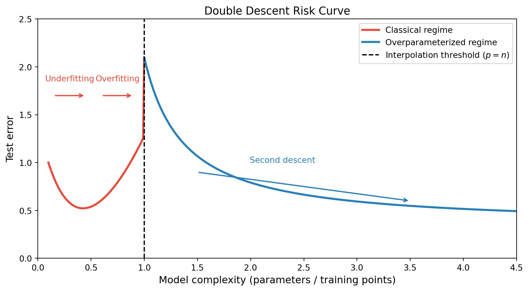
• Belkin et al. (2019) demonstrated that for many model classes, the risk curve has two descents separated by a peak at the interpolation threshold

Schematic double descent risk curve. The classical regime (left of threshold) follows the U-curve. The modern overparameterized regime (right) shows a second descent.

The key insight: classical theory only shows the left side of this picture. Modern large models operate far to the right. The risk at infinite complexity is often lower than the classical optimal!

Observing double descent empirically

Double descent in a linear model with random Fourier features. At the interpolation threshold (n features = n data points), test error peaks. Adding more features—using the minimum-norm solution—drives error back down.

This is a real numerical experiment, not a schematic. We use random Fourier features—each feature is cos(2π f_j x + φ_j) for a random frequency and phase. As we add more features: - Fewer than n=50: model can’t fit the data → high bias - Near 50: exactly fitting, poorly conditioned → high variance (the spike) - More than 50: lstsq returns the minimum-norm solution → smooth interpolant → lower error

The minimum-norm solution acts as implicit regularization.

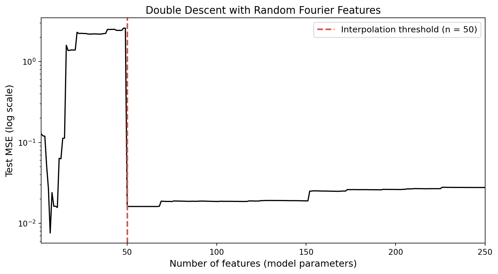
Piecewise linear fits at increasing K

Piecewise linear models at K=5, 12, 33, and 255 features fitted to the same noisy data. K=5 underfits; K=33 is near the interpolation threshold and wildly oscillates; K=255 interpolates all points yet remains smooth—the second descent.

This data comes from the MLU-Explain double descent visualization. The same noisy dataset is fit at four complexity levels. K=5 cannot capture the signal (underfitting). K=12 is still in the classical regime—fit is improving. K=33 is right at the interpolation threshold (n ≈ p): the model can exactly pass through every point, but only in a violently oscillatory way—variance explodes. K=255 is overparameterized: the minimum-norm solution spreads weight smoothly and generalizes well despite interpolating every training point.

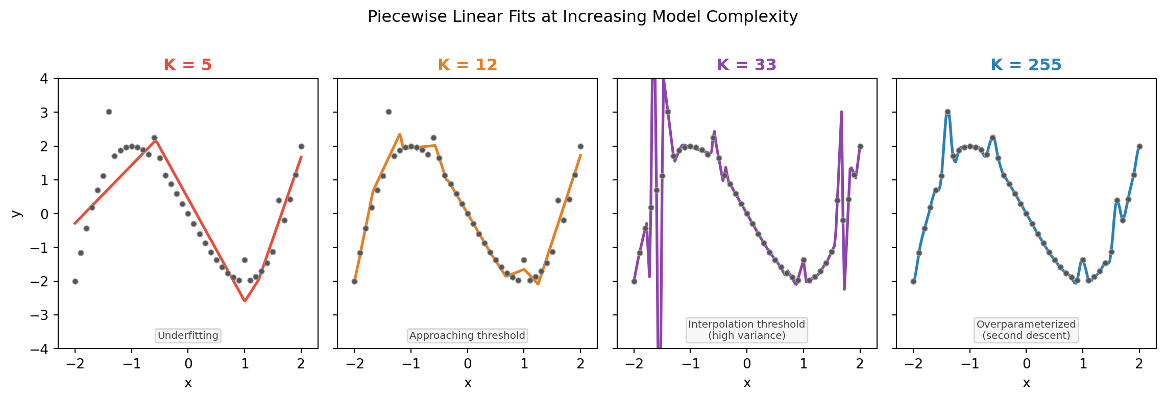
Why Does the Second Descent Happen?

• In the overparameterized regime, there are infinitely many interpolating solutions
• The minimum-norm solution (returned by gradient descent / pseudoinverse) has an implicit regularization property:
  • It minimizes \(\|\boldsymbol{\theta}\|_2\) subject to fitting the training data
  • This is equivalent to ridge regression in the limit \(\lambda \to 0^+\)
  • It does not fit the noise dimensions beyond what is needed

\[\hat{\boldsymbol{\theta}}^+ = \arg\min_{\boldsymbol{\theta}} \|\boldsymbol{\theta}\|_2 \quad \text{s.t.} \quad \mathbf{X}\boldsymbol{\theta} = \mathbf{y}\]

This is the key theoretical result (Bartlett et al., 2020; Hastie et al., 2022). The minimum-norm solution has small norm, which means it doesn’t amplify noise. Gradient descent on overparameterized linear models initialized at zero always converges to this solution.

The implicit regularization arises from the geometry of the solution space, not from an explicit penalty term. This is a profound insight: the algorithm itself provides regularization in the overparameterized regime.

Implicit regularization connects back to binding

• In the binding system, the minimum-norm solution is the \((k_\text{on}, k_\text{off})\) pair closest to the origin consistent with the measured \(K_d\)
• All solutions on the manifold predict equally—the min-norm solution does not “waste” parameter magnitude on unobserved directions
• In ML, overparameterized models similarly distribute weight across many directions; the minimum-norm solution is the smoothest interpolant

We’re completing the analogy. The binding system gave us intuition about a 2-parameter model where only 1 combination is constrained. Machine learning models may have millions of parameters where only a tiny fraction of directions in weight space matter. The minimum-norm solution is benign because it has no reason to put weight in unobserved directions.

Universal Approximation

From Linear to Nonlinear Models

• Everything above applies to linear models (linear in features)
• Neural networks are nonlinear: the features themselves are learned from data
• The same overparameterization argument extends—but with far greater expressive power

The Universal Approximation Theorem

Theorem (Hornik et al., 1989; Cybenko, 1989): A feedforward network with a single hidden layer containing a sufficient number of neurons with a non-polynomial activation function can approximate any continuous function on a compact subset of \(\mathbb{R}^n\) to arbitrary precision.

• This means: given enough neurons, a neural network can represent any target function
• However, it says nothing about:
  • How many neurons are “enough”
  • Whether gradient descent will find the right weights
  • Whether the model will generalize from finite data

UAT is an existence result. It is like knowing that a solution to an equation exists—it doesn’t tell you how to find it or whether the solution you find will be the right one. The next lecture addresses what makes neural networks actually work in practice.

A preview: overparameterized neural networks also show double descent

• Modern neural networks are massively overparameterized (often \(p \gg n\) by factors of \(10^3\)–\(10^6\))
• Like linear models, they interpolate training data and still generalize
• The implicit regularization comes from:
  • Stochastic gradient descent (SGD) dynamics
  • Early stopping
  • Architecture choices
• Next lecture: what does it take for neural networks to actually work?

The teaser. Double descent in neural networks has been demonstrated empirically by Belkin et al. (2019) and studied theoretically in the “neural tangent kernel” (NTK) regime. The practical takeaways come next.

Review

Further Reading

• Belkin M. et al. Reconciling modern machine-learning practice and the bias-variance trade-off. PNAS, 2019.
• Bartlett P. et al. Benign overfitting in linear regression. PNAS, 2020.
• Zhang C. et al. Understanding deep learning requires rethinking generalization. ICLR, 2017.
• Hastie T. et al. Surprises in High-Dimensional Ridgeless Least Squares Interpolation. Ann. Statist., 2022.

Review Questions

1. In the binding kinetics example, we cannot determine \(k_\text{on}\) and \(k_\text{off}\) individually from equilibrium data. Why can we still make accurate predictions about binding occupancy?
2. What is the interpolation threshold? What does classical bias-variance theory predict happens to test error there?
3. Describe the double descent phenomenon in words. How does it contradict the classical picture?
4. What is the minimum-norm solution, and why does gradient descent find it for overparameterized linear models?
5. How is the minimum-norm solution related to ridge regression? What happens as \(\lambda \to 0\)?
6. A colleague says: “Your model has more parameters than training points—it must be overfitting.” How would you respond using the concepts from this lecture?
7. The Universal Approximation Theorem says a sufficiently large network can approximate any continuous function. Why is this an existence result rather than a practical recipe?
8. If a model achieves zero training error but low test error, what does this tell you about the model and the data?
9. How does overparameterization in neural networks differ from overparameterization in linear models with random features?
10. A drug discovery team trains a neural network on 500 compounds. They argue that using a 10-million-parameter model will overfit. What questions would you ask before agreeing or disagreeing?