Partial Least Squares Regression

Aaron Meyer & Yosuke Tanigawa (based on slides from Pam Kreeger)

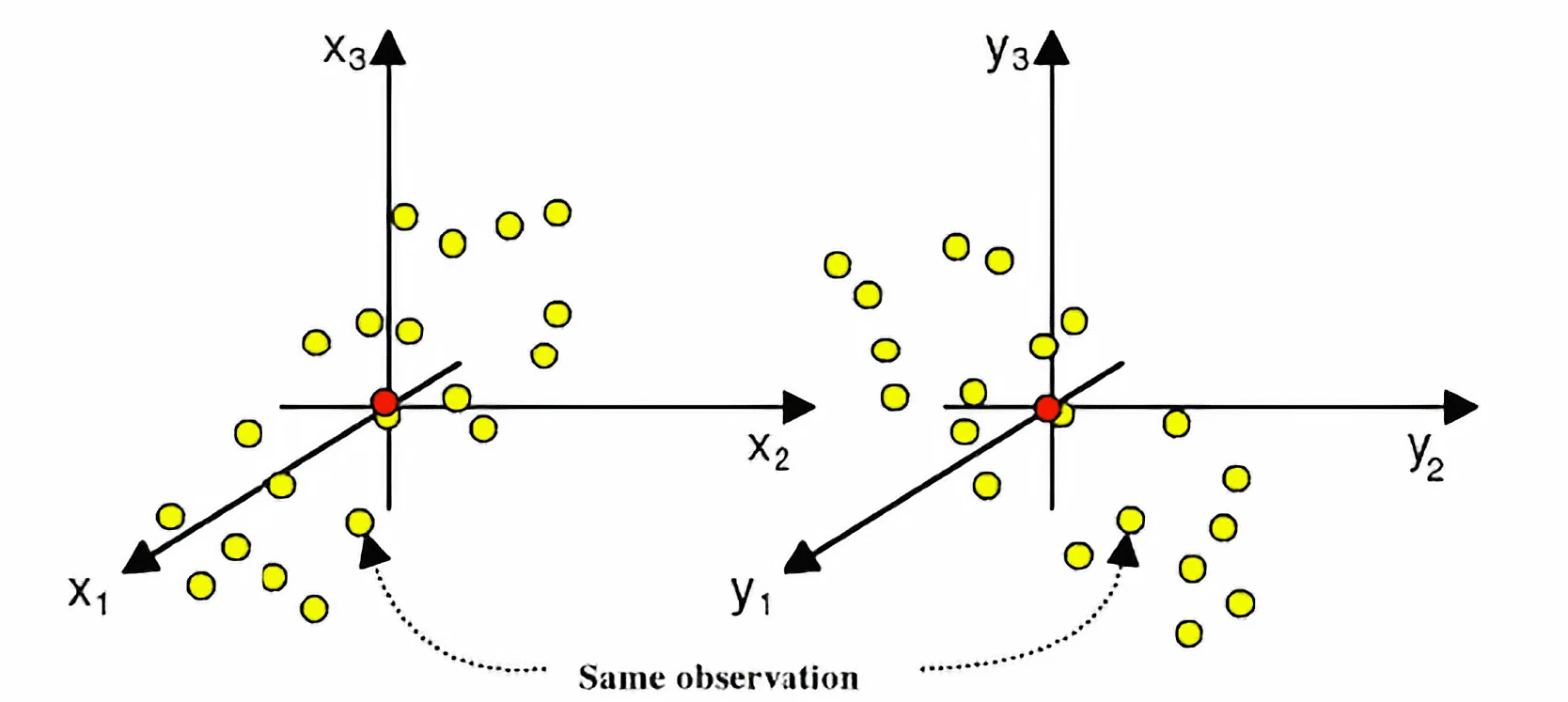
Common challenge: Finding coordinated changes within data

Diagram from Lee et al. showing the challenge of finding coordinated changes in complex biological data.
Bar chart or heatmap showing how the timing and order of drug treatment affects cell death percentage.

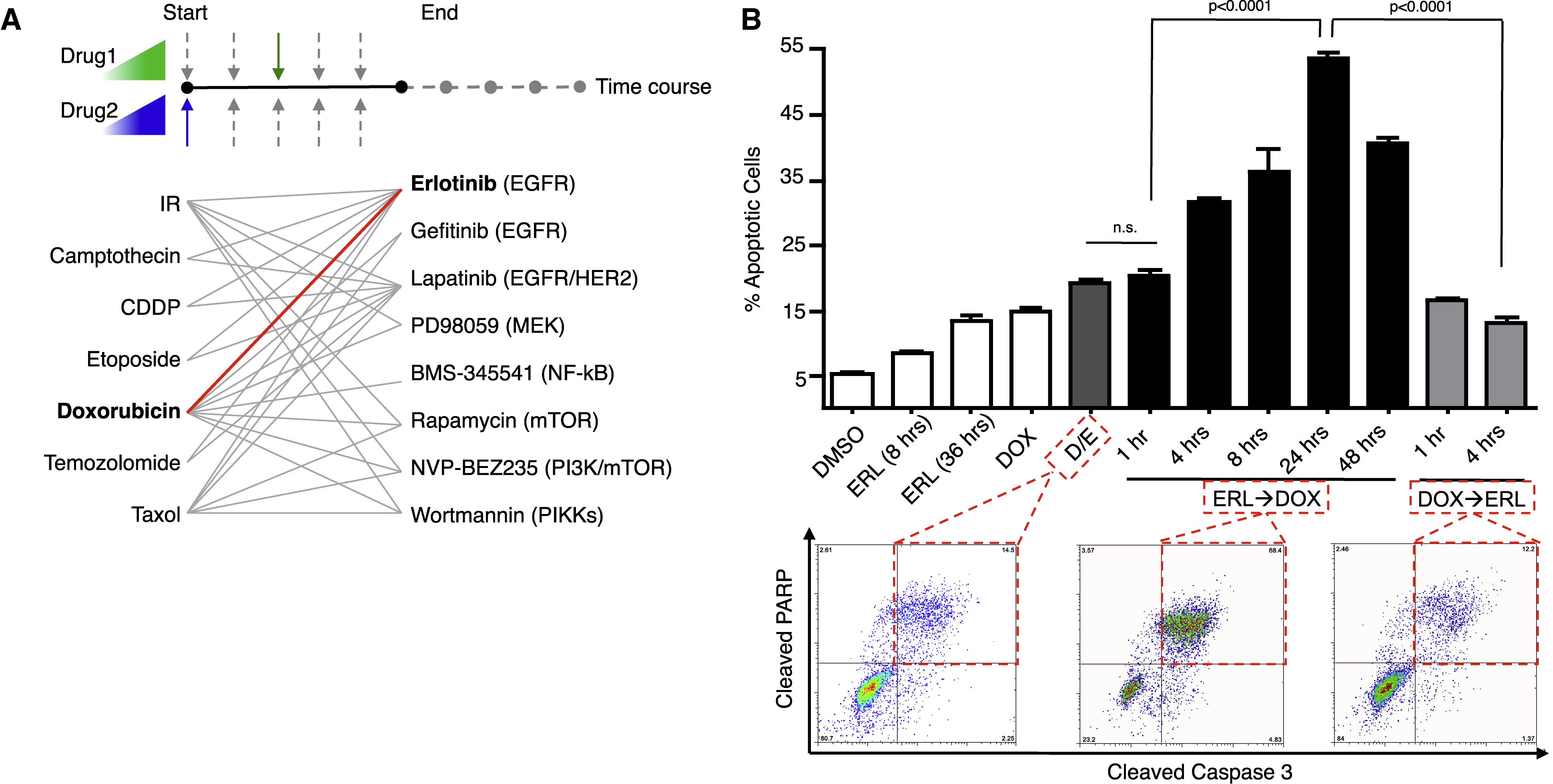
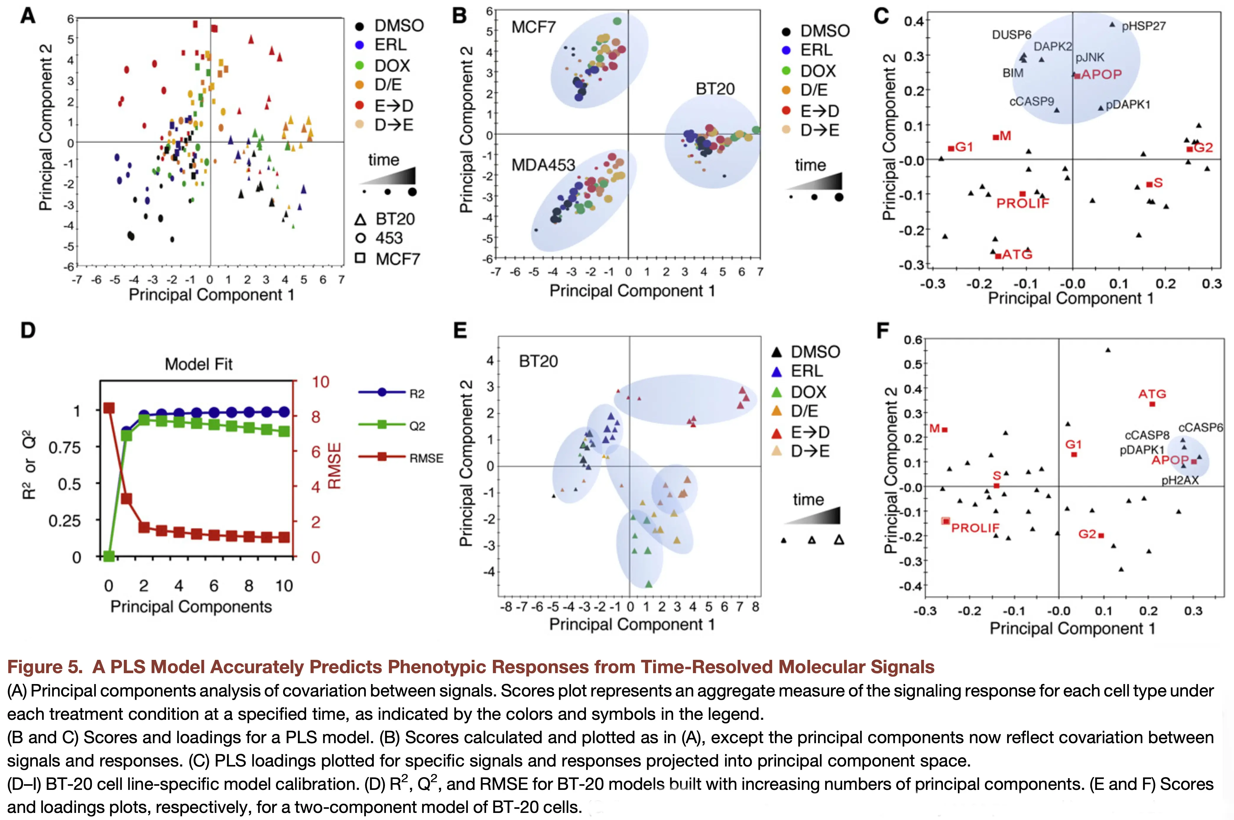
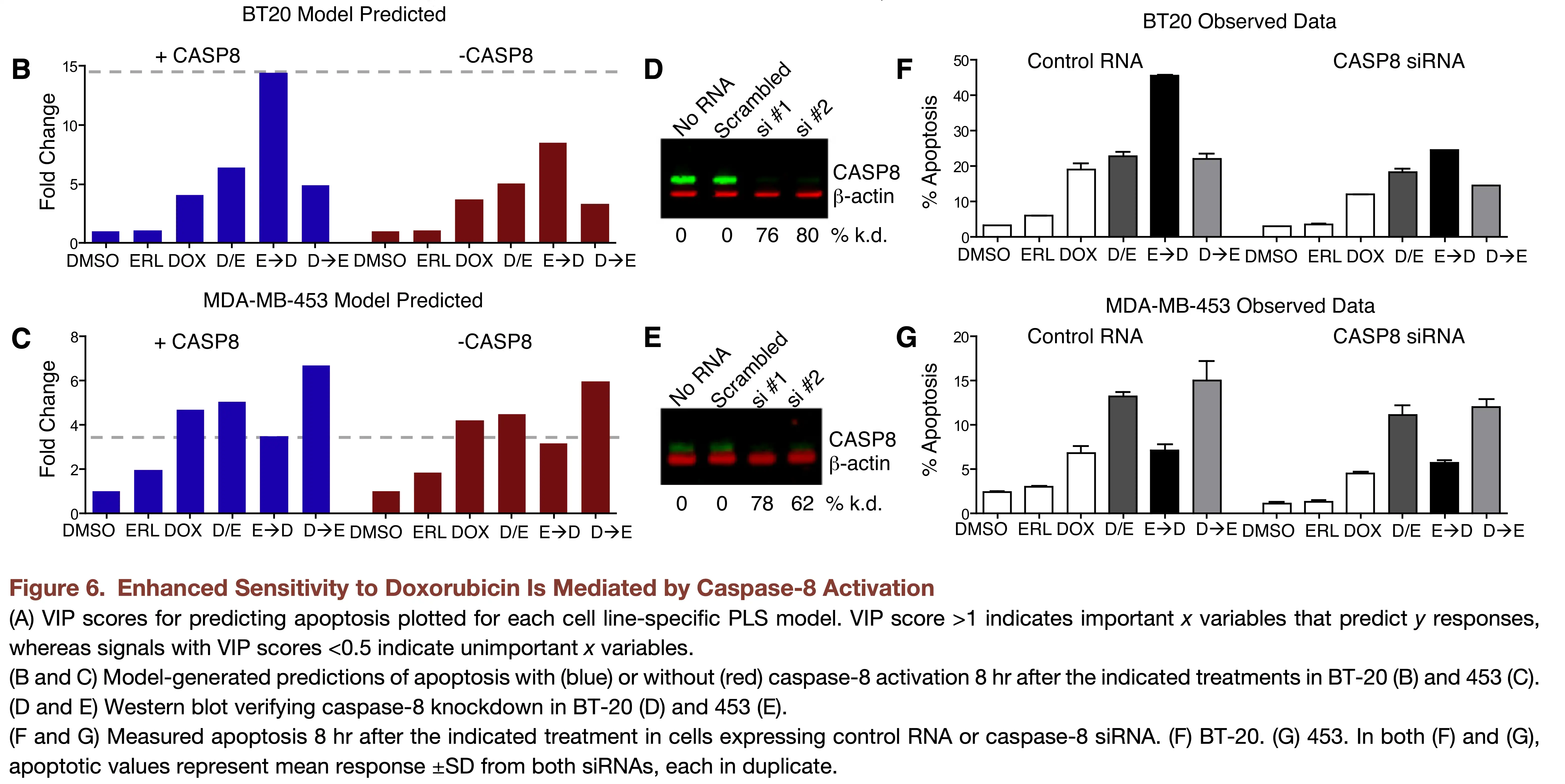
The timing and order of drug treatment affects cell death.

Figure from Lee et al. likely showing the experimental setup or results related to drug combinations.

Notes about the methods today

  • We will cover two related methods today: principal components regression (PCR) and partial least squares regression (PLSR).
  • Both methods are used for supervised prediction; however, they have a number of distinct properties from other methods we will discuss.
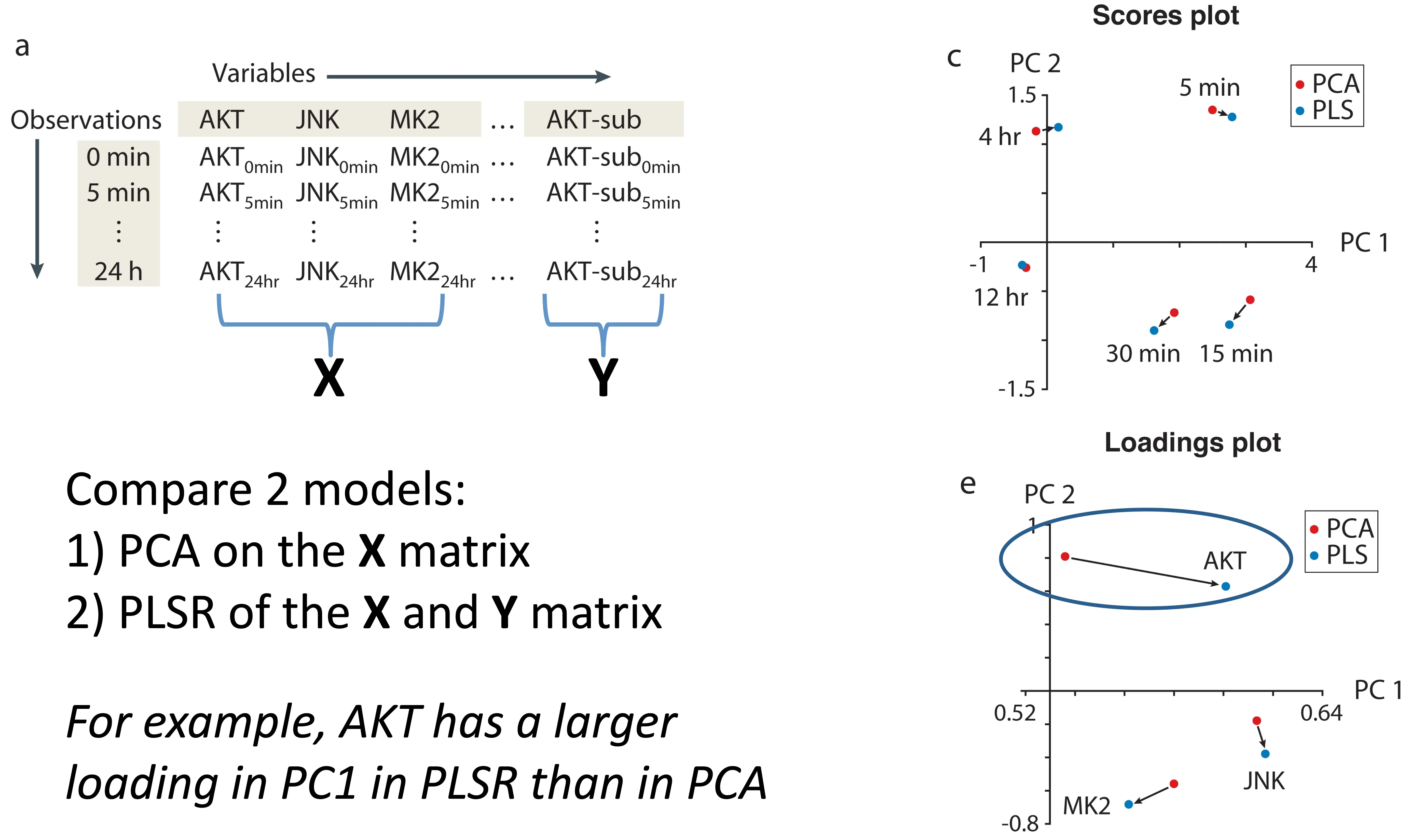
  • PCR constructs components using only \(\mathbf{X}\), while PLSR uses information from both \(\mathbf{X}\) and \(\mathbf{Y}\) when constructing latent directions.
  • Learning about PLSR is more difficult than it should be, partly because papers describing it span areas of chemistry, economics, medicine and statistics, with differences in terminology and notation.

Regularization

  • Both PCR and PLSR can act as forms of regularization.
  • Reduce the dimensionality of our regression problem to \(N_{\textrm{comp}}\) components.
  • Prioritize certain variance in the data.

Principal Components Regression (PCR)

Core idea

One solution: use the concepts from PCA to reduce dimensionality.

First step: Simply apply PCA!

Dimensionality goes from \(m\) to \(N_{\textrm{comp}}\).

Principal Components Regression

  1. Decompose the \(\mathbf{X}\) matrix (scores \(\mathbf{T}\), loadings \(\mathbf{P}\), residuals \(\mathbf{E}_X\)):

\[ \mathbf{X} = \mathbf{T}\mathbf{P}^\top + \mathbf{E}_X \]

  1. Regress \(\mathbf{Y}\) against the scores (scores describe observations, so they link \(\mathbf{X}\) and \(\mathbf{Y}\) for each observation)

\[ \mathbf{Y} = \mathbf{T}\mathbf{B} + \mathbf{E}_Y \]

How do we determine the right number of components to use for our prediction?

A remaining potential problem

  • The PCs for the \(\mathbf{X}\) matrix do not necessarily capture variation in \(\mathbf{X}\) that is important for \(\mathbf{Y}\).
  • Standard PCR can struggle when predictive signal lies in lower-variance directions.
  • There are a few developments around PCR that aim to improve prediction or interpretability.

Recent developments around PCR (advanced topics)

pcLasso: the LASSO meets PCR

  • pcLasso is a supervised regression method that combines sparsity with shrinkage toward leading principal-component directions.
  • It can be helpful when predictors are highly correlated and we want both good prediction and a smaller, more interpretable set of features.

Supervised PCA

  • Supervised PCA uses association with \(\mathbf{Y}\) to select features before performing PCA and regression.
  • It can help when many features are irrelevant to prediction.

Partial Least Squares Regression (PLSR)

The core idea of PLSR

What if, instead of choosing components based only on variance in \(\mathbf{X}\), we choose latent directions that maximize the covariance between scores derived from \(\mathbf{X}\) and \(\mathbf{Y}\)?

What is covariance?

Covariance measures how two variables vary together:

\[ \mathrm{cov}(x, y) = \frac{1}{n-1}\sum_{i=1}^{n}(x_i - \bar{x})(y_i - \bar{y}) \]

PLSR is a cross-decomposition method

We will find latent components for both \(\mathbf{X}\) and \(\mathbf{Y}\):

\[ \mathbf{X} = \mathbf{T}\mathbf{P}^\top + \mathbf{E} \]

\[ \mathbf{Y} = \mathbf{U}\mathbf{Q}^\top + \mathbf{F} \]

Diagram of PLSR as a cross-decomposition method, showing X decomposing into T and P, and Y decomposing into U and Q, with a relationship between T and U.

Algorithm to find PLSR solutions

  • Iterative minimization while exchanging scores
  • NIPALS: nonlinear iterative partial least squares

NIPALS while exchanging the scores

Step 1: Take a random column of \(\mathbf{Y}\) to be \(\mathbf{u}_a\), and regress it against \(\mathbf{X}\).

\[ \mathbf{w}_a = \dfrac{1}{\mathbf{u}_a^\top\mathbf{u}_a} \cdot \mathbf{X}_a^\top\mathbf{u}_a \]

Flowchart or diagram illustrating the iterative steps of the NIPALS algorithm for Partial Least Squares.

https://learnche.org/pid/latent-variable-modelling/projection-to-latent-structures/how-the-pls-model-is-calculated

Step 2: Normalize \(\mathbf{w}_a\).

\[ \mathbf{w}_a = \dfrac{\mathbf{w}_a}{\sqrt{\mathbf{w}_a^\top \mathbf{w}_a}} \]

Flowchart or diagram illustrating the iterative steps of the NIPALS algorithm for Partial Least Squares.

https://learnche.org/pid/latent-variable-modelling/projection-to-latent-structures/how-the-pls-model-is-calculated

Step 3: Regress \(\mathbf{w}_a\) against \(\mathbf{X}_a\) to obtain \(\mathbf{t}_a\).

\[ \mathbf{t}_a = \dfrac{1}{\mathbf{w}_a^\top\mathbf{w}_a} \cdot \mathbf{X}_a\mathbf{w}_a \]

Flowchart or diagram illustrating the iterative steps of the NIPALS algorithm for Partial Least Squares.

https://learnche.org/pid/latent-variable-modelling/projection-to-latent-structures/how-the-pls-model-is-calculated

Step 4: Regress \(\mathbf{t}_a\) against \(\mathbf{Y}_a\) to obtain \(\mathbf{c}_a\).

\[ \mathbf{c}_a = \dfrac{1}{\mathbf{t}_a^\top\mathbf{t}_a} \cdot \mathbf{Y}_a^\top\mathbf{t}_a \]

Flowchart or diagram illustrating the iterative steps of the NIPALS algorithm for Partial Least Squares.

https://learnche.org/pid/latent-variable-modelling/projection-to-latent-structures/how-the-pls-model-is-calculated

Step 5: Regress \(\mathbf{c}_a\) against \(\mathbf{Y}_a\) to obtain \(\mathbf{u}_a\).

\[ \mathbf{u}_a = \dfrac{1}{\mathbf{c}_a^\top\mathbf{c}_a} \cdot \mathbf{Y}_a\mathbf{c}_a \]

Flowchart or diagram illustrating the iterative steps of the NIPALS algorithm for Partial Least Squares.

https://learnche.org/pid/latent-variable-modelling/projection-to-latent-structures/how-the-pls-model-is-calculated

Step 6: Cycle until convergence

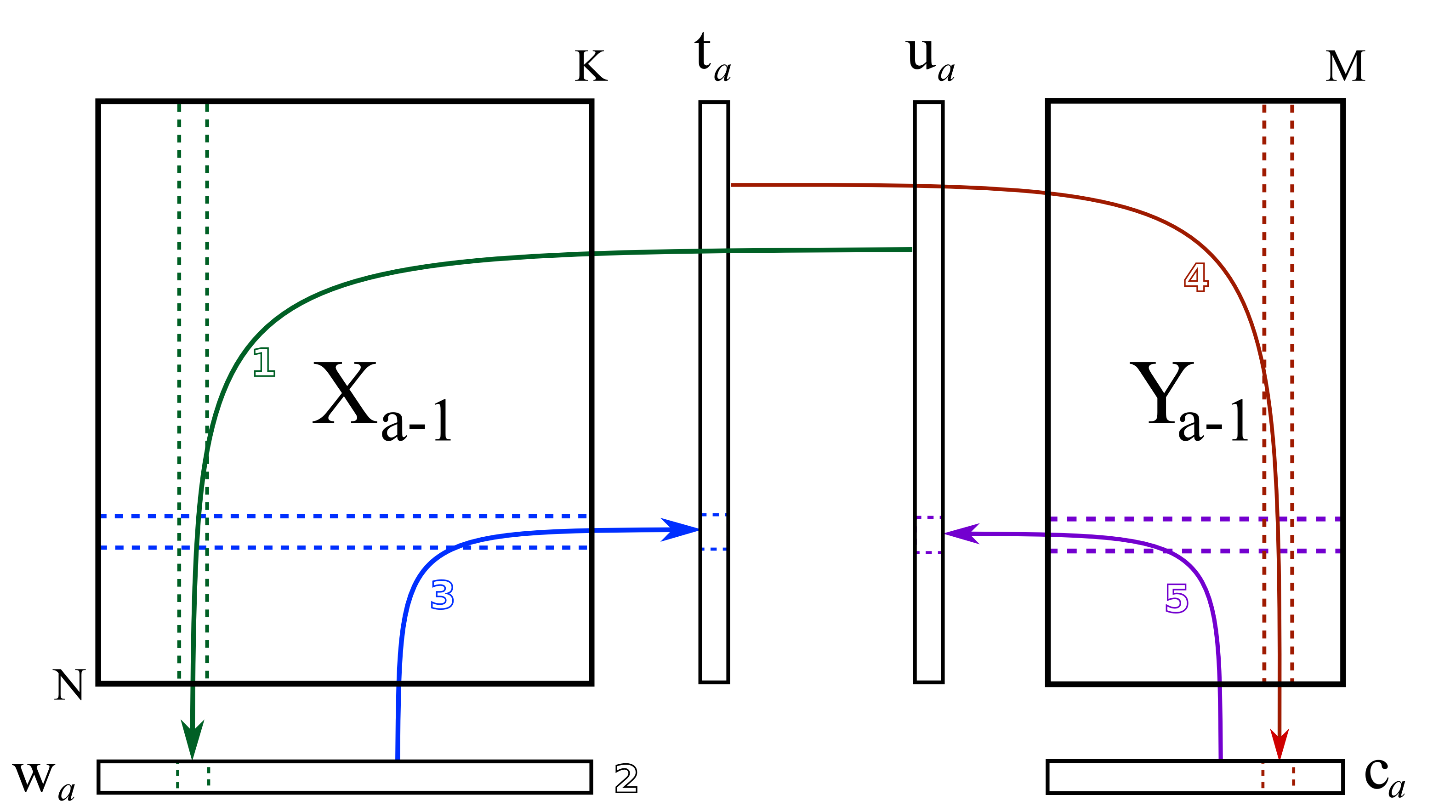
Cycle until convergence, then subtract off the variance explained by \(\widehat{\mathbf{X}}_a = \mathbf{t}_a\mathbf{p}_a^\top\) and \(\widehat{\mathbf{Y}}_a = \mathbf{t}_a \mathbf{c}_a^\top\).

Flowchart or diagram illustrating the iterative steps of the NIPALS algorithm for Partial Least Squares.

https://learnche.org/pid/latent-variable-modelling/projection-to-latent-structures/how-the-pls-model-is-calculated

Components in PLSR and PCA Differ

Figure from Janes et al (2006) comparing the principal components derived from PCA and PLSR, showing how they capture different variance.

Janes et al, Nat Rev MCB, 2006

Determining the Number of Components

\(R^2X\) provides the variance explained in \(\mathbf{X}\):

\[ R^2X = 1 - \frac{\left\Vert \mathbf{X}_{\textrm{PLSR}} - \mathbf{X} \right\Vert_F^2}{\left\Vert \mathbf{X} \right\Vert_F^2} \]

\(R^2Y\) shows the variance explained in \(\mathbf{Y}\):

\[ R^2Y = 1 - \frac{\left\Vert \mathbf{Y}_{\textrm{PLSR}} - \mathbf{Y} \right\Vert_F^2}{\left\Vert \mathbf{Y} \right\Vert_F^2} \]

If you are trying to predict something, you should look at the cross-validated \(R^2Y\) (a.k.a. \(Q^2Y\)).

PLSR uncovers coordinated cell death mechanisms

Figure from Lee et al. showing how PLSR helps uncover coordinated cell death mechanisms.
Additional figure from Lee et al. illustrating the results of PLSR analysis on cell death mechanisms.

Practical Notes

PCR

PLSR

  • sklearn.cross_decomposition.PLSRegression
    • Uses M.fit(X, Y) to train
    • Can use M.predict(X) to get new predictions
    • PLSRegression(n_components=3) to set the number of components at initialization
    • Or M.n_components = 3 after initialization, followed by refitting the model

Comparison: PLSR vs. PCR

PCR

  • Uses PCA as an initial decomposition step, then is just normal linear regression
  • PCA maximizes the variance explained in the independent (X) data
  • Useful if you want to capture unbiased structure in X and it is aligned with biological variations you care about

PLSR

  • Chooses components to maximize covariance between latent scores derived from \(\mathbf{X}\) and \(\mathbf{Y}\)
  • Takes into account both the dependent (Y) and independent (X) data
  • Useful to capture subtle but coordinated biological effect

Performance of PLSR

  • PLSR can be very effective for prediction, especially when predictors are highly correlated and the signal is low-dimensional
    • This is incredibly powerful, especially when the response depends on coordinated variation spread across many correlated features
  • Interpreting why PLSR predicts something can be challenging

Review

Which method would you use?

  • We will consider several hypothetical scenarios involving datasets \(\mathbf{X}\) and \(\mathbf{Y}\).
  • For each scenario, decide which method you would try:
    • PCA: principal component analysis for unsupervised dimensionality reduction
    • OLS: ordinary least squares regression
    • Lasso: sparse linear regression with an \(l_1\) penalty
    • PCR: principal components regression
    • PLSR: partial least squares regression

Scenario 1: Single-cell RNA-seq (cell type discovery)

You have:

  • \(\mathbf{X}\): gene expression (20,000 genes \(\times\) 5,000 cells)
  • \(\mathbf{Y}\): coarse labels (e.g., “treated” vs “control”)
  • Goal: understand major sources of variation and visualize cell populations

Which would you use: PCA, OLS, Lasso, PCR, or PLSR? Why?

Scenario 2: Drug response prediction (high-dimensional, correlated features)

You have:

  • \(\mathbf{X}\): gene expression (10,000 genes \(\times\) 200 cell lines)
  • \(\mathbf{Y}\): drug sensitivity (continuous IC50)
  • Goal: predict drug response from high-dimensional molecular measurements
  • Predictive signal is weak but spread across many correlated genes

Which would you use: PCA, OLS, Lasso, PCR, or PLSR? Why?

Scenario 3: Clinical outcome with noisy labels

You have:

  • \(\mathbf{X}\): proteomics data (500 proteins \(\times\) 80 patients)
  • \(\mathbf{Y}\): an electronic health record (EHR)-derived inflammation score aggregated from multiple hospitals and measurement pipelines
  • Goal: build a robust predictor despite substantial outcome noise
  • Small sample size

Which would you use: PCA, OLS, Lasso, PCR, or PLSR? Why?

Scenario 4: Sparse biomarker model

You have:

  • \(\mathbf{X}\): gene expression (5,000 genes \(\times\) 150 samples)
  • \(\mathbf{Y}\): expression level of a developmental marker gene
  • Goal: predict marker expression with a small, interpretable set of regulators
  • You believe only a small number of upstream regulators are truly important, and you want an interpretable predictive model

Which would you use: PCA, OLS, Lasso, PCR, or PLSR? Why?

Scenario 5: Hidden low-variance biology

You have:

  • \(\mathbf{X}\): metabolomics data (300 metabolites \(\times\) 120 samples)
  • \(\mathbf{Y}\): subtle treatment effect
  • Goal: detect and predict a weak biological effect hidden by stronger background variation
  • Treatment effect is small compared to diet/environment variation

Which would you use: PCA, OLS, Lasso, PCR, or PLSR? Why?

Reading & Resources

Review Questions

  1. What are three differences between PCA and PLSR in implementation and application?
  2. What is the difference between PCR and PLSR? When does this difference matter more/less?
  3. How might you need to prepare your data before using PLSR?
  4. How can you determine the right number of components for a model?
  5. What feature of biological data makes PLSR/PCR useful relative to direct regularization approaches (LASSO/ridge)?
  6. Can you apply K-fold cross-validation to a PLSR model? If so, when do you scale your data?
  7. Can you apply bootstrapping to a PLSR model? Describe what this would look like.
  8. You use the same X data but want to predict a different Y variable. Do your X loadings change in your new model? What about for PCR?