Fitting & Regression Redux, Regularization

Aaron Meyer & Yosuke Tanigawa (based on slides from Rob Tibshirani)

Outline

• Example
• The Bias-Variance Tradeoff
• Ridge Regression
• The LASSO
• Comparing LS, Ridge, and the LASSO
• Review

Example

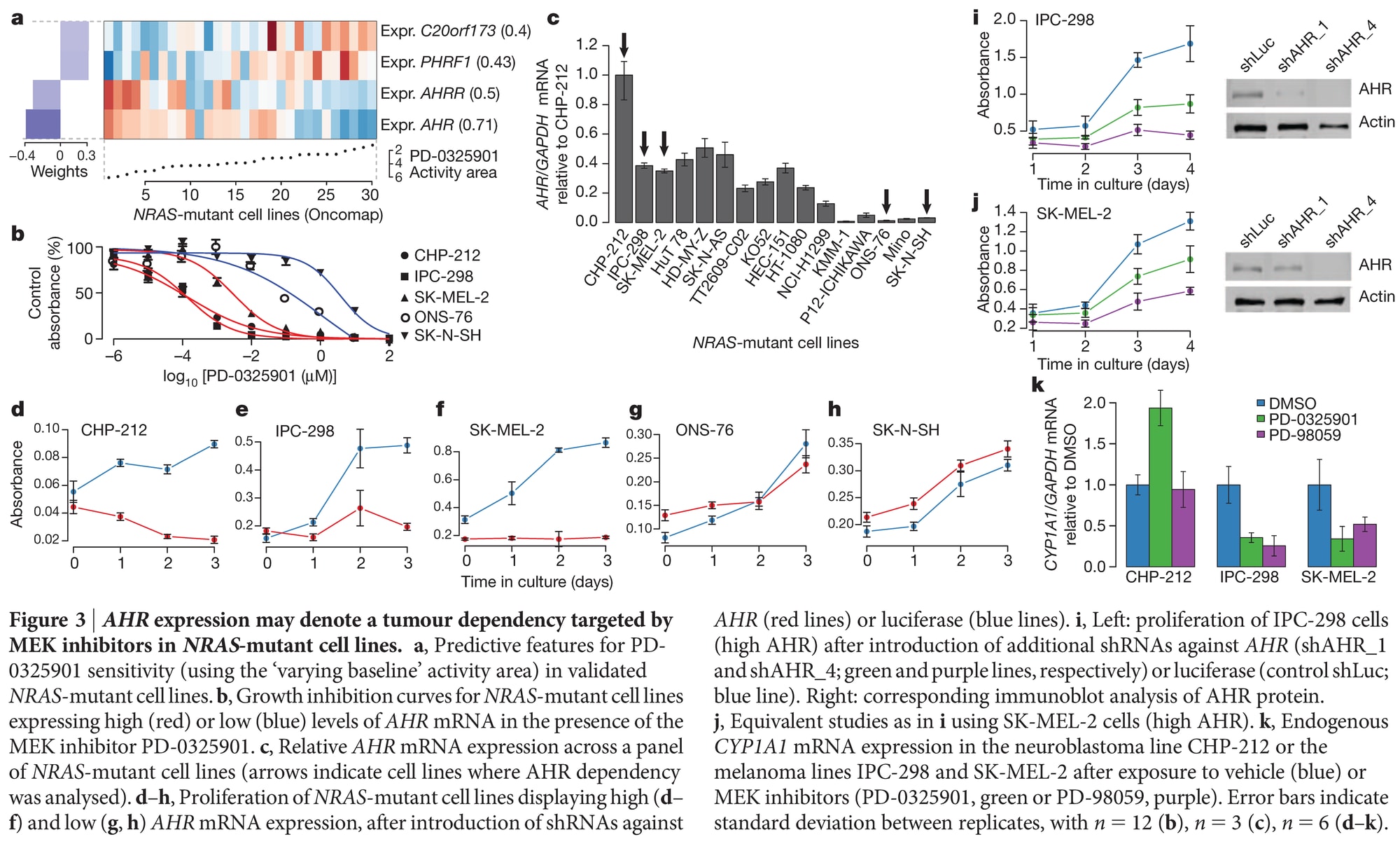
Predicting Drug Response

The Bias-Variance Tradeoff

Estimating \(\boldsymbol{\beta}\)

• As usual, we assume the model: \[y=f(\mathbf{z})+\epsilon, \epsilon\sim N(0,\sigma^2I)\]
• In regression analysis, our major goal is to come up with some good regression function \[\hat{f}(\mathbf{z}) = \mathbf{z}^\top \hat{\boldsymbol{\beta}}\]
• So far, we’ve been dealing with \(\hat{\boldsymbol{\beta}}^{ls}\), or the least squares solution:
  • \(\hat{\boldsymbol{\beta}}^{ls}\) has well-known properties (e.g., Gauss-Markov, ML)
• But can we do better?

Choosing a good regression function

• Suppose we have an estimator \[\hat{f}(\mathbf{z}) = \mathbf{z}^\top \hat{\boldsymbol{\beta}}\]
• To see if this is a good candidate, we can ask ourselves two questions:
  1. Is \(\hat{\boldsymbol\beta}\) close to the true \(\boldsymbol{\beta}\)?
  2. Will \(\hat{f}(\mathbf{z})\) fit future observations well?
• These might have very different outcomes!!

Is \(\hat{\boldsymbol{\beta}}\) close to the true \(\boldsymbol{\beta}\)?

• To answer this question, we might consider the mean squared error of our estimate \(\hat{\boldsymbol{\beta}}\):
  • i.e., consider squared distance of \(\hat{\boldsymbol{\beta}}\) to the true \(\boldsymbol{\beta}\): \[\textrm{MSE}(\hat{\boldsymbol{\beta}}) = \mathop{\mathbb{E}}\left[\lVert \hat{\boldsymbol{\beta}} - \boldsymbol{\beta} \rVert^2\right] = \mathop{\mathbb{E}}[(\hat{\boldsymbol{\beta}} - \boldsymbol{\beta})^\top (\hat{\boldsymbol{\beta}} - \boldsymbol{\beta})]\]
• Example: In least squares (LS), we know that: \[\mathrm{MSE}(\hat{\boldsymbol{\beta}}^{ls}) = \mathop{\mathbb{E}}[(\hat{\boldsymbol{\beta}}^{ls} - \boldsymbol{\beta})^\top (\hat{\boldsymbol{\beta}}^{ls} - \boldsymbol{\beta})] = \sigma^2 \mathrm{tr}[(\mathbf{Z}^\top \mathbf{Z})^{-1}]\]

Mean squared error of the least squares fit

\[\mathrm{MSE}(\hat{\boldsymbol{\beta}}^{ls}) = \sigma^2 \mathrm{tr}[(\mathbf{Z}^\top \mathbf{Z})^{-1}]\]

Interpretation:

• \(\sigma^2\): the magnitude of noise in the linear model
• \((\mathbf{Z}^\top \mathbf{Z})^{-1}\): Sensitivity to the design matrix. Poorly conditioned or highly correlated predictors will lead to large MSE
• \(\mathrm{tr}[(\mathbf{Z}^\top \mathbf{Z})^{-1}]\): Total variance across all coefficients

Recall the linear model: \(\mathbf{y} = \mathbf{Z}\boldsymbol\beta + \boldsymbol\epsilon, \quad \boldsymbol\epsilon \sim N(0, \sigma^2 \mathbf{I})\)

The least squares estimator is: \(\hat{\boldsymbol{\beta}}^{ls} = (\mathbf{Z}^\top \mathbf{Z})^{-1} \mathbf{Z}^\top \mathbf{y}\)

Under these assumptions, the estimator has distribution: \[\hat{\boldsymbol{\beta}}^{ls} \sim \mathcal{N}\left(\boldsymbol{\beta},\; \sigma^2 (\mathbf{Z}^\top \mathbf{Z})^{-1}\right)\]

We define the mean squared error: \(\mathrm{MSE}(\hat{\boldsymbol{\beta}}) = \mathbb{E}\left[\|\hat{\boldsymbol{\beta}} - \boldsymbol{\beta}\|^2\right]\)

Let \(\mathbf{x} = \hat{\boldsymbol{\beta}}^{ls} - \boldsymbol{\beta}\). Since the estimator is unbiased, \(\mathbb{E}[\mathbf{x}] = 0\), and \(\mathrm{MSE} = \mathbb{E}[\mathbf{x}^\top \mathbf{x}]\)

A useful identity for zero-mean vectors: \[\mathbb{E}[\mathbf{x}^\top \mathbf{x}] = \mathrm{tr}(\mathrm{Cov}(\mathbf{x}))\]

Applying this: \[\mathrm{MSE}(\hat{\boldsymbol{\beta}}^{ls}) = \mathrm{tr}\left(\mathrm{Cov}(\hat{\boldsymbol{\beta}}^{ls})\right) = \sigma^2 \mathrm{tr}\left((\mathbf{Z}^\top \mathbf{Z})^{-1}\right)\]

Will \(\hat{f}(\mathbf{z})\) fit future observations well?

• Just because \(\hat{f}(\mathbf{z})\) fits our data well does not mean that it will fit new data well
  • In fact, suppose that we take new measurements \(y_i'\) at the same \(\mathbf{z}_i\)’s: \[(\mathbf{z}_1,\mathbf{y}_1'),(\mathbf{z}_2,\mathbf{y}_2'), \ldots ,(\mathbf{z}_n,\mathbf{y}_n')\]
  • So if \(\hat{f}(\cdot)\) is a good model, then \(\hat{f}(\mathbf{z}_i)\) should also be close to the new target \(y_i'\)
• This motivates prediction error (PE)

Have students draw lines for smoking vs. heart attack risk over data. Make two datasets to explain variance.

Prediction error and the bias-variance tradeoff

• Good estimators should, on average, have small prediction errors
• Let’s consider the PE at a particular target point \(\mathbf{z}_0\):
  • \(\mathrm{PE}(\mathbf{z}_0) = \sigma_{\epsilon}^2 + \textrm{Bias}^2(\hat{f}(\mathbf{z}_0)) + \textrm{Var}(\hat{f}(\mathbf{z}_0))\), where
  • \(\textrm{Bias}(\hat{f}(\mathbf{z}_0)) = \mathbb{E}[\hat{f}(\mathbf{z}_0)] - f(\mathbf{z}_0)\)
  • \(\textrm{Var}(\hat{f}(\mathbf{z}_0)) = \mathbb{E}\left[(\hat{f}(\mathbf{z}_0) - \mathbb{E}[\hat{f}(\mathbf{z}_0)])^2\right]\)
• Such a decomposition is known as the bias-variance tradeoff

• Not going to derive, but comes directly from the definitions

Bias-variance tradeoff

\[ \mathrm{PE}(\mathbf{z}_0) = \sigma_{\epsilon}^2 + \textrm{Bias}^2(\hat{f}(\mathbf{z}_0)) + \textrm{Var}(\hat{f}(\mathbf{z}_0)) \]

• As model becomes more complex (more terms included), local structure/curvature is picked up
• But coefficient estimates suffer from high variance as more terms are included in the model
• So introducing a little bias in our estimate for \(\boldsymbol{\beta}\) might lead to a large decrease in variance, and hence a substantial decrease in PE
  • We’ll cover a few well-known techniques

Bias-variance decomposition and Prediction Error (PE)

We start from the regression model:

\[ y = f(\mathbf{z}) + \epsilon, \quad \epsilon \sim (0, \sigma^2I) \]

Our goal is to understand how well a fitted model \(\hat{f}\) will predict new data.

Let \(D\) denote the training data used to fit the model. At a new point \(\mathbf{z}_0\),

\[ \mathrm{PE}(\mathbf{z}_0) = \mathbb{E}_{D,\epsilon}\left[(y_0 - \hat{f}_D(\mathbf{z}_0))^2\right]. \]

Since \(y_0 = f(\mathbf{z}_0) + \epsilon\), we have \(\mathrm{PE}(\mathbf{z}_0) = \mathbb{E}_{D,\epsilon}\left[(f(\mathbf{z}_0) + \epsilon - \hat{f}_D(\mathbf{z}_0))^2\right].\)

Expanding the square gives

\[ \mathrm{PE}(\mathbf{z}_0) = \mathbb{E}_{D,\epsilon}\left[(f(\mathbf{z}_0) - \hat{f}_D(\mathbf{z}_0))^2\right] + \mathbb{E}[\epsilon^2] + 2\mathbb{E}_{D,\epsilon}\left[\epsilon \bigl(f(\mathbf{z}_0) - \hat{f}_D(\mathbf{z}_0)\bigr)\right]. \]

The cross term is zero because \(\epsilon\) has mean zero and is independent of the training data, so \(\mathbb{E}_{D,\epsilon}\left[\epsilon \bigl(f(\mathbf{z}_0) - \hat{f}_D(\mathbf{z}_0)\bigr)\right] = 0.\)

Therefore,

\[ \mathrm{PE}(\mathbf{z}_0) = \sigma^2 + \mathbb{E}_D\left[(f(\mathbf{z}_0) - \hat{f}_D(\mathbf{z}_0))^2\right]. \]

Define

• \(\mathrm{Bias}(\hat{f}(\mathbf{z}_0)) = \mathbb{E}_D[\hat{f}_D(\mathbf{z}_0)] - f(\mathbf{z}_0)\), and
• \(\mathrm{Var}(\hat{f}(\mathbf{z}_0)) = \mathbb{E}_D\left[\left(\hat{f}_D(\mathbf{z}_0) - \mathbb{E}_D[\hat{f}_D(\mathbf{z}_0)]\right)^2\right].\)

We have the bias-variance tradeoff:

\[ \mathrm{PE}(\mathbf{z}_0) = \sigma^2 + \mathrm{Bias}^2 + \mathrm{Var}. \]

• \(\sigma^2\) is irreducible noise.
• Bias is systematic error from model misspecification
• Variance is sensitivity to the training data

Bias term is squared, so a small amount is often acceptable if it reduces variance enough.

Depicting the bias-variance tradeoff

A graph depicting the bias-variance tradeoff.

• Regularization can be anything.
• Today we’ll see two/three examples.

Ridge Regression

Ridge regression: \(l_2\) penalty as regularization

• If the \(\beta_j\)’s are unconstrained…
  • They can explode
  • And hence are susceptible to very high variance
• To control variance, we might regularize the coefficients
  • i.e., we might control how large the coefficients grow
• Might impose the ridge constraint (both equivalent):
  • minimize \(\sum_{i=1}^n (y_i - \boldsymbol{\beta}^\top \mathbf{z}_i)^2\: \mathrm{s.t.} \sum_{j=1}^p \beta_j^2 \leq t\)
  • minimize \((\mathbf{y} - \mathbf{Z}\boldsymbol{\beta})^\top (\mathbf{y} - \mathbf{Z}\boldsymbol{\beta})\: \mathrm{s.t.} \sum_{j=1}^p \beta_j^2 \leq t\)
• By convention (very important):
  • Z is assumed to be standardized (mean 0, unit variance)
  • y is assumed to be centered

Penalized residual sum of squares (PRSS)

• Can write the ridge constraint as the following penalized residual sum of squares (PRSS):

\[ \begin{aligned} \textrm{PRSS}(\boldsymbol{\beta})_{\ell_2} &= \sum_{i=1}^{n}(y_i - \mathbf{z}_i^{\top}\boldsymbol{\beta})^2 + \lambda\sum_{j=1}^{p}\beta_j^2 \\ &= (\mathbf{y} - \mathbf{Z}\boldsymbol{\beta})^{\top}(\mathbf{y} - \mathbf{Z}\boldsymbol{\beta}) + \lambda{\left\|\boldsymbol{\beta}\right\|}_2^2 \end{aligned} \]

• Its solution may have smaller average PE than \(\hat{\boldsymbol{\beta}}^{ls}\)
• \(\textrm{PRSS}(\boldsymbol{\beta})_{\ell_2}\) is convex, and hence has a unique solution
• Taking derivatives, we obtain: \[\frac{\delta \textrm{PRSS}(\boldsymbol{\beta})_{\ell_2}}{\delta \boldsymbol{\beta}} = -2\mathbf{Z}^\top (\mathbf{y}-\mathbf{Z}\boldsymbol{\beta})+2\lambda\boldsymbol{\beta}\]

• So this is just an added term to OLS!
• Ask if folks have seen convex before.
• What happens with \(\lambda\) going to infinity?
• How about \(\lambda\) going to 0?
• Often software might ask for \(log(\lambda)\) or \(1/\lambda\). Be sure to check.

The ridge solutions

• The solution to \(\textrm{PRSS}(\hat{\boldsymbol{\beta}})_{\ell_2}\) is now seen to be: \[\hat{\boldsymbol{\beta}}_\lambda^{ridge} = (\mathbf{Z}^\top \mathbf{Z} + \lambda \mathbf{I}_p)^{-1} \mathbf{Z}^\top \mathbf{y}\]
  • Remember that Z is standardized
  • y is centered
• \(\lambda\) makes the problem non-singular even if \(\mathbf{Z}^\top \mathbf{Z}\) is not invertible
  • Was the original motivation for ridge (Hoerl & Kennard, 1970)
• Solution is indexed by the tuning parameter \(\lambda\)

• As simple to compute as OLS!
• How do we figure out the tuning parameter?
• What does the invertibility statement mean? We can solve even when p > n!

Ridge coefficient paths

• The \(\lambda\) values trace out a set of ridge solutions, as illustrated below

Ridge coefficient path for the diabetes data set found in the lars library in R.

Tuning parameter \(\lambda\)

• Notice that the solution is indexed by the parameter \(\lambda\)
  • For each value of \(\lambda\), we obtain a solution
  • Varying \(\lambda\) gives a series of solutions
• \(\lambda\) is the shrinkage parameter
  • \(\lambda\) controls the amount of regularization
  • As \(\lambda\) decreases to 0, we recover the least squares solution
  • As \(\lambda\) becomes very large, the coefficients shrink toward 0 (intercept-only model if \(\mathbf{y}\) is centered)

A few notes on ridge regression

• Ridge regression decreases the effective degrees of freedom of the model
  • It can still be fit when \(p > n\), but the effective complexity stays below the unregularized case
• This can be shown by examination of the smoother matrix
  • We won’t do this—it’s a complicated argument

Choosing \(\lambda\)

• We need to tune \(\lambda\) to minimize the mean squared error
  • This is part of the bigger problem of model selection
• In their original paper, Hoerl and Kennard introduced ridge traces:
  • Plot the components of \(\hat{\beta}_\lambda^{ridge}\) against \(\lambda\)
  • Choose \(\lambda\) for which the coefficients are not rapidly changing and have “sensible” signs
  • No objective basis; heavily criticized by many

K-fold cross-validation

• A common method to determine \(\lambda\) is K-fold cross-validation.

Plot of CV errors and standard error bands

Cross validation errors from a ridge regression example on spam data.

The LASSO

The LASSO: \(l_1\) penalty

• Tibshirani (J. Roy. Stat. Soc. B, 1996) introduced the LASSO: least absolute shrinkage and selection operator
• LASSO coefficients are the solutions to the \(l_1\) optimization problem: \[\mathrm{minimize}\: (\mathbf{y}-\mathbf{Z}\boldsymbol{\beta})^\top (\mathbf{y}-\mathbf{Z}\boldsymbol{\beta})\: \mathrm{s.t.} \sum_{j=1}^p \lVert \beta_j \rVert \leq t\]
• This is equivalent to the penalized loss function: \[PRSS(\boldsymbol{\beta})_{\ell_1} = \sum_{i=1}^n (y_i - \mathbf{z}_i^\top \boldsymbol{\beta})^2 + \lambda \sum_{j=1}^p \lVert \beta_j \rVert\] \[\quad = (\mathbf{y}-\mathbf{Z}\boldsymbol{\beta})^\top (\mathbf{y}-\mathbf{Z}\boldsymbol{\beta}) + \lambda\lVert \boldsymbol{\beta} \rVert_1\]

• Date shows the difficulty in solving.
• \(l_1\) indicates the sum of absolute values.
• So \(l_2\) norm is more sensitive to large values. Here, sensitive to all values.
• What happens if \(\hat{\beta}_j\) doesn’t really affect the fitting quality?

\(\lambda\) (or t) as a tuning parameter

• Again, we have a tuning parameter \(\lambda\) that controls the amount of regularization
• One-to-one correspondence with the threshold t:
  • recall the constraint: \[\sum_{j=1}^p \lVert \beta_j \rVert \leq t\]
  • Hence, have a “path” of solutions indexed by \(t\)
  • If \(t_0 = \sum_{j=1}^p \lVert \hat{\beta}_j^{ls} \rVert\) (equivalently, \(\lambda = 0\)), we obtain no shrinkage (and hence obtain the LS solutions as our solution)
  • Often, the path of solutions is indexed by a fraction of shrinkage factor of \(t_0\)

• Software will implement this in different ways.

Sparsity and exact zeros

• Often, we believe that many of the \(\beta_j\)’s should be 0
• Hence, we seek a set of sparse solutions
• Large enough \(\lambda\) (or small enough t) will set some coefficients exactly equal to 0!
  • So LASSO will perform model selection for us!

Computing the LASSO solution

• Unlike ridge regression, \(\hat{\boldsymbol{\beta}}^{lasso}_{\lambda}\) has no simple closed-form expression
• Original implementation involves quadratic programming techniques from convex optimization
• LARS (least angle regression) computes a closely related path efficiently
  • Efron et al., Ann. Statist., 2004 proposed LARS
  • With a small modification, LARS can also be used to compute the LASSO path
• Forward stagewise is a closely related method and is straightforward to implement
  • https://doi.org/10.1214/07-EJS004

Forward stagewise algorithm

• As usual, assume Z is standardized and y is centered
• Choose a small step size \(\epsilon\). The forward-stagewise algorithm then proceeds as follows:
  1. Start with initial residual \(\mathbf{r}=\mathbf{y}\), and \(\beta_1=\beta_2=\ldots=\beta_p=0\)
  2. Find the predictor \(\mathbf{Z}_j (j=1,\ldots,p)\) most correlated with r
  3. Update \(\beta_j=\beta_j+\delta_j\), where \(\delta_j = \epsilon\cdot \mathrm{sign}\langle\mathbf{r},\mathbf{Z}_j\rangle = \epsilon\cdot \mathrm{sign}(\mathbf{Z}_j^\top \mathbf{r})\)
  4. Set \(\mathbf{r}=\mathbf{r} - \delta_j \mathbf{Z}_j\)
  5. Repeat from step 2 many times

• We may skip the forward stagewise algorithm.

Comparing LS, Ridge, and the LASSO

Constraint geometry

• Even though \(\mathbf{Z}^{\top}\mathbf{Z}\) may not be of full rank, both ridge regression and the LASSO admit solutions
• We have a problem when \(p \gg n\) (more predictor variables than observations)
  • But both ridge regression and the LASSO have solutions
  • Regularization tends to reduce prediction error

Estimation picture for the lasso (left) and ridge regression (right).

• The residual sum of squares has elliptical contours.
• The least squares estimate is at the center of the contours.
• The diamond (\(l_1\)) and the disk (\(l_2\)) represent the constraint regions.
• Solutions at the corners of the diamond represent sparse solutions.

The LASSO, LARS, and Forward Stagewise paths

Comparison of the LASSO, LARS, and Forward Stagewise coefficient paths for the diabetes data set.

More comments on variable selection

• Now suppose \(p \gg n\)
  • Of course, we would like a parsimonious model (Occam’s Razor)
• Ridge regression produces coefficient values for each of the \(p\) predictors
• But because of its \(l_1\) penalty, the LASSO will set many of the variables exactly equal to 0!
  • That is, the LASSO produces sparse solutions
• So LASSO takes care of model selection for us
  • And we can even see when variables jump into the model by looking at the LASSO path

Variants of the Ridge and the LASSO

• Zou and Hastie (2005) propose the elastic net, which combines ridge and the LASSO penalties
  • Paper asserts that the elastic net can improve error over LASSO
  • Still produces sparse solutions
  • The strengths and balance of the \(l_2\) (ridge) and the \(l_1\) (LASSO) penalties are both tunable hyperparameters
• Tay, Friedman, and Tibshirani (2019) propose principal components lasso (pcLasso), which is a generalization of elastic net
  • It also has a connection to principal component regression
  • We will cover principal component regression in Partial Least Squares Regression lectures

• Write out penalized error with all three norms (error, \(l_1\), \(l_2\))

High-dimensional data and underdetermined systems

Why high-dimensional problems are underdetermined

• In many modern data analysis problems, we have \(p \gg n\)
  • These comprise “high-dimensional” problems
• When fitting the model \(y = \mathbf{z}^\top \boldsymbol{\beta}\), we can have many solutions
  • i.e., our system is underdetermined
• Reasonable to suppose that most of the coefficients are exactly equal to 0

But do these methods pick the right/true variables?

• Suppose that only \(S\) elements of \(\boldsymbol{\beta}\) are non-zero
• Now suppose we had an “Oracle” that told us which components of \(\boldsymbol{\beta} = (\beta_1,\beta_2,\ldots,\beta_p)\) are truly non-zero
• Let \(\boldsymbol{\beta}^{*}\) be the least squares estimate of this “ideal” estimator:
  • So \(\boldsymbol{\beta}^{*}\) is 0 in every component that \(\boldsymbol{\beta}\) is 0
  • The non-zero elements of \(\boldsymbol{\beta}^{*}\) are computed by regressing \(\mathbf{y}\) on only the \(S\) important covariates
• It turns out we can get quite close to this cheating solution without cheating!
  • Candès & Tao, Ann. Statist., 2007.

Implementation

• The notebook can be found on the course website.

Review

Further Reading

• Computer Age Statistical Inference, Chapter 16
• sklearn: Linear Models
• Candès E. and Tao T. The Dantzig selector: statistical estimation when p is much larger than n.

Review Questions

1. What is the bias-variance tradeoff? Why might we want to introduce bias into a model?
2. What is regularization? What are some reasons to use it?
3. What is the difference between ridge regression and LASSO? How should you choose between them?
4. Are you guaranteed to find the global optimal answer for ridge regression? What about LASSO?
5. What is variable selection? Which method(s) perform it? What can you say about the answers?
6. What does it mean when one says ridge regression and LASSO give a series of solutions?
7. What can we say about the relationship between fitting error and prediction error?
8. What does regularization do to the variance of a model?
9. A colleague tells you about a new form of regularization they’ve come up with (e.g., force all parameters to be within the range 1–3). How would this influence the variance of the model? Might this improve the prediction error?
10. Can you regularize NNLS? If so, how could you implement this?